Compression refrigeration cycles
Introduction
In a power cycle, heat is provided to produce mechanical energy. A refrigeration cycle operates in reverse: it receives mechanical energy which is used to raise the temperature level of heat.
Technological explanations are given in these pages :
Introduction
We have presented the principle of operation of these cycles in the first part of the lightweight presentation, and we have studied in Guided Exploration S-M3-V9 some possible settings of the simple refrigeration cycle.
Let us recall also that the useful energy of a refrigeration cycle is the heat extracted from the evaporator, and the purchased energy is the work provided to the compressor. As the ratio of the two is generally greater than 1, the term efficiency is no longer suitable, and this is why we speak of the cycle coefficient of performance (COP).
Although the problem of optimizing refrigeration cycles is very different from that of power cycles, in both cases we seek to minimize irreversibilities, so that the approaches meet.
To fix ideas, consider a refrigeration cycle intended to cool to a temperature of -10 °C a cold enclosure placed in a room at 20 °C.

T2 = - 10 °C = 263.15 K
T1 – T2 = 30 °C
COP = 263.15/30 = 8.8
Reverse Carnot COP is 8.8.
In practice, the thermodynamic fluid evolves between temperatures T1 = 75 °C and T2 = -20 °C approximately, which corresponds to a COP equal to 253.15/95 = 3.7, much lower than the theoretical value of 8.8.
In the cycles that we have studied so far, the refrigerant evaporation pressure was equal to 1.78 bar, which allowed a cold chamber to be cooled slightly below 0 °C. Such a value is acceptable for a simple refrigerator, but not for a fridge-freezer, the temperature of the cold enclosure of which must be at least -15 °C.
We will therefore use a much lower evaporation pressure, equal to 1 bar, for our reference cycle. For the rest, we will keep the settings of Guided Exploration S-M3-V9: superheat 5 °C, subcooling -10 °C, with the proviso that the compressor isentropic efficiency will be 0.8.
The reference cycle that we consider is then given in the synoptic view of the figure below.
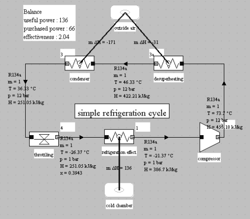
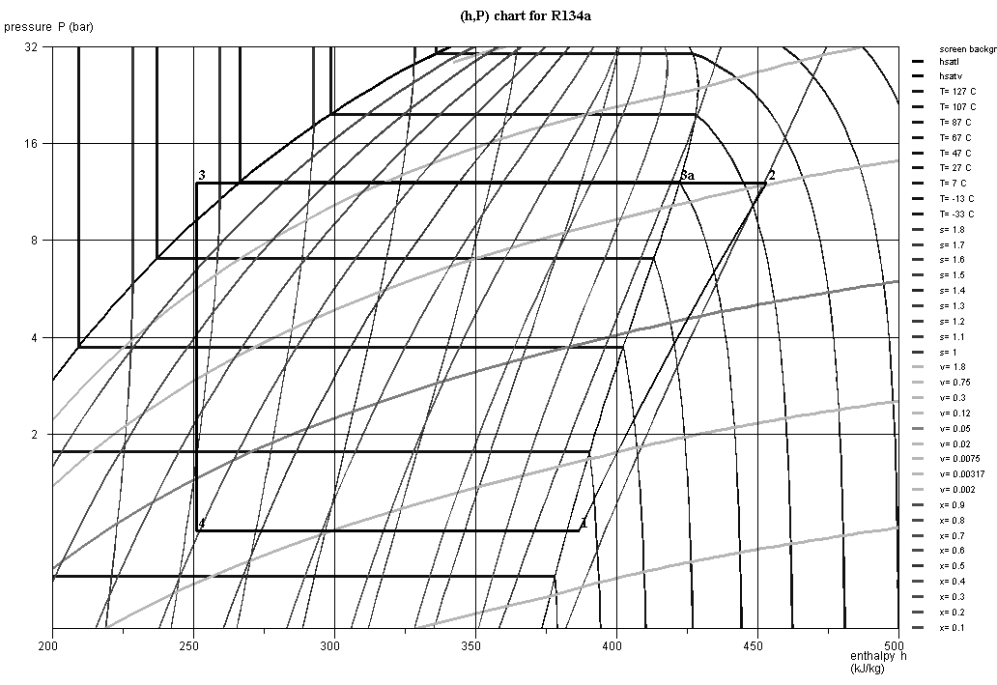
The evaporation and condensation pressures are 1 and 12 bar. Its COP is worth 2.04. Its plot in the (h, ln(P)) chart in the figure below.
Two-stage cycles
To improve the refrigeration cycles, we are also led on the one hand to minimize the irreversibilities coming from temperature heterogeneities both outside the system and internally, and on the other hand to use staged compression.
The expressions of the reverse Carnot cycle show that the value of the COP deteriorates when the temperature difference (T1 - T2) increases.
It is clear that the value of COP is greater the smaller the difference (T1 - T2).
When this difference increases, the compression ratio increases accordingly, which has the effect of:
lowering the isentropic efficiency;
increasing the compressor outlet temperature to very high values, with the risk of oil decomposition.
We know that staged compression with intercooling can reduce compression work.
This complication of the cycle is justified when the temperature difference (T1 - T2) increases.
In practice, as soon as the compression ratio exceeds 6, the single-stage cycle reaches its limits and must be replaced by multi-stage cycles. In most cases, the refrigeration systems are two-stage.
We know that, when it is necessary to fractionate a compression, it can be advantageous to cool the fluid between two stages. Cooling can be ensured by the condenser external heat source, or another cooler if exists.
Consider our reference cycle, i.e. with subcooling of 10 °C and 5 °C superheat, working between 1 and 12 bar (Figures above). Its COP is equal to 2, the refrigeration effect being 135.6 kJ/kg, and the compression work 66.5 kJ/ kg.
Consider what can be done by using a staged compression. The compression ratio being equal to 12, the intermediate pressure can be chosen equal to 3.5 bar at first guess.
Maintaining an isentropic efficiency equal to 0.8, the compression end temperature is equal to 23.6 °C, that is to say just above that of condenser cooling air (assumed to be at 20 °C).
With intermediate cooling from 24 °C to 10 °C, the COP is slightly improved and passes to 2.1 (Figure below). The gain is low, and this cycle will not work without an additional heat sink.

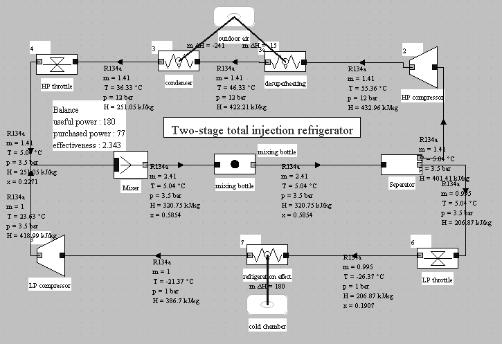
To ensure both the internal cooling of the vapors exiting the low pressure compressor, and also increase in the vaporization plateau, it is interesting to stage the expansion. The simplest and most effective cycle is called a total injection cycle or refrigeration cycle with flash chamber (Figure below).

In this cycle, vapor exiting the LP compressor and two-phase fluid leaving the HP expansion valve are mixed in a bottle which acts like a capacitor and a separator, the vapor being sucked into the HP compressor, while the liquid phase passes through the LP expansion valve.
Total injection refrigeration installation (exploration C-M3-V3)
In this guided exploration, you will see how a total injection two-stage compression cycle can be modeled.
You will learn how to set a phase separator and a mixer.
Important note: to make this page easier for you to read, we have inserted here these guided explorations, but you should use the ones contained in the Thermoptim browser installed on your computer, because it is them that are coupled with Thermoptim and all the corresponding working files.
This results in a significant improvement of the refrigeration cycle, whose COP reaches 2.34, which is 17% better than that of the single-stage cycle (Figure below).
The refrigeration effect is 180 kJ/kg, and the compression work 76.8 kJ/kg. The compression work is more important than in the basic cycle, because of the circulation, in the HP cycle, of a mass flow rate (1.4 kg/s) greater than in the LP cycle (1 kg/s).
The figure below shows the plot of this cycle in the (h, ln(P)) chart.

