Introduction
We have seen that, when it is necessary to split a compression, it can be advantageous to cool the fluid between two stages. When a refrigeration cycle has to operate with a high compression ratio, a variant of the basic cycle is precisely to do this.
In order to be able on the one hand to internally cool the vapors leaving the low pressure compressor, and on the other hand to increase the vaporization plateau, it is advantageous to also split the expansion. The simplest and most efficient cycle is called the total injection cycle.
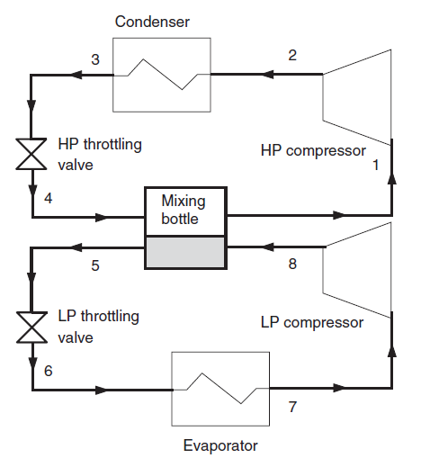
In this cycle, vapor exiting the LP compressor and two-phase fluid leaving the HP expansion valve are mixed in a bottle which acts like a capacitor and a separator, the vapor being sucked into the HP compressor, while the liquid phase passes through the LP expansion valve.
Reference cycle
Consider that the reference cycle for R134a operates between an evaporation pressure of 1 bar and a condenser pressure of 12 bar.
At the outlet of the evaporator, a flow rate of fluid is entirely vaporized, with an overheating of 5 °C.
It is then compressed to 12 bar following an irreversible adiabatic compression. The actual compression is characterized by an isentropic efficiency, defined as the ratio of the work of the reversible compression to the real work. Its value is assumed to be 0.8.
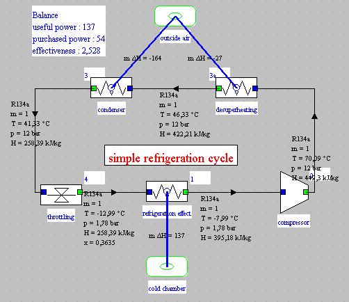
The cooling of the fluid in the condenser by exchange with the outside air involves two stages: desuperheating in the vapor zone followed by condensation, with sub-cooling of 10 °C.
It is then expanded without work in a capillary, to the pressure of 1 bar.
The COP for such a cycle is worth 2.04.
Settings retained for the total injection cycle
The total injection refrigeration cycle operates between an evaporation pressure of 1 bar and a condenser pressure of 12 bar, the intermediate pressure being 3.5 bar.
At the outlet of the evaporator, the flow rate of fluid is entirely vaporized, with an overheating of 5 °C.
It is then compressed to 3.5 bar in the LP compressor following an irreversible adiabatic compression, characterized by an isentropic efficiency assumed to be equal to 0.8.
The compressed vapor is directed to the mixing bottle, into which also enters the two-phase fluid leaving the HP throttling valve. In the bottle, the two phases of the mixture separate, the liquid phase being directed to the LP throttling valve which feeds the evaporator, while the vapor phase is sucked by the HP compressor where it is compressed up to 12 bar, the efficiency isentropic assumed to be 0.8.
We have already studied the configuration of a phase separator. It does not pose any particular problem, the distribution of the flow entering the two outlet branches being made in proportion to the quality in vapor.
Cooling the vapor in the condenser by exchange with the outside air involves two stages: desuperheating in the vapor zone followed by condensation.
The liquid is then expanded without work to the pressure of 3.5 bar, then directed to the mixing bottle.
In our model, we set the flow rate in the evaporator at the value of 1 g/s. The flow in the HP circuit, which is calculated by the separator, is 1.41 g/s.
The balance of the cycle shows a significant improvement in the COP which reaches the value of 2.34, or 17% better than that of the single-stage cycle. The cooling capacity is also increased, from 136 W to 180 W, due to the fact that the evaporator input quality is much lower.
Loading the model
We will now study the total injection refrigeration cycle..
Load the model
Click on the following link: Open a file in Thermoptim
You can also:
- either open the "Project files/Example catalog" (CtrlE) and select model m11.1 in Chapter 11 model list.
- or directly open the diagram file (refrig2stageTotInj.dia) using the "File/Open" menu in the diagram editor menu, and the project file (refrig2stageTotInj.prj) using the "Project files/Load a project" menu in the simulator.
Study of the influence of subcooling
Cycle plot in the (h, ln (P)) chart
First step: loading the R134a (h, ln (P)) chart
Click this button
You can also open the diagram using the "Interactive Diagrams" line in the "Special" menu of the simulator screen, which opens an interface that links the simulator and the diagram. Double-click in the field at the top left of this interface to choose the type of diagram desired (here "Vapors")..
Once the diagram is open, choose "R134a" from the substance menu, and select "(h, p)" from the "Chart" menu.
Second step: loading a pre-recorded cycle corresponding to the loaded project
Click this button
- in the diagram window, choose "Load a cycle" from the Cycle menu
- and select "refrig2stSR10Thin.txt" from the list of available cycles.
- Then click on the "Connected points" line in the Cycle menu.
The cycle appears in blue. A distinction is made between the two LP and HP circuits.
Simple cycle overlay
Click this button
- in the diagram window, choose "Load a cycle" from the Cycle menu
- and select "refrig112R134a.txt" from the list of available cycles.
- Then click on the "Connected points" line in the Cycle menu.
Variation in performance when the intermediate pressure varies
In the initial configuration we chose an intermediate pressure of 3.5 bar.
You will now vary this pressure to study the influence of this parameter on cycle performance.
To do this, you must enter the new pressure in points 4a, 9 and 4, each time and recalculate each of these points.
Then recalculate several times in the simulator screen until the balance stabilizes.
You can see that, depending on whether you want to favor a high COP or a high power, the optimal intermediate pressure is not the same.
Conclusion
This exploration allowed you to study a two-stage total injection cycle model for a refrigeration installation, more complex than a simple cycle.
Several variants of two-stage cycles exist in addition to the one we have presented here.
The loading of the simple cycle plotted in black makes it possible to superimpose it on the cycle with total injection. In the diagram (h, ln (P)), the increase in the cooling effect is clearly visible.