Cryogenics
Cryogenic Cycles
The term cryogenics is used to describe methods of refrigeration at very low temperatures (typically below 125 K), and distinguish them from ordinary refrigeration cycles. Many of these methods relate to the liquefaction of gases known as permanent, like air, natural gas, hydrogen or helium.
Cryogenics is the fi eld of engineering that focuses on systems operating at very low temperature, which poses special problems, particularly in terms of fluids and materials.
Refrigeration and cryogenic liquefaction cycles involve combinations of paraisothermal compressions, cooling, thermal regeneration, and isenthalpic or adiabatic expansion of fluids.
There are four major families of cryogenic thermodynamic processes:
isenthalpic expansion Joule-Thomson processes;
isentropic expansion reverse Brayton cycles;
mixed processes involving isenthalpic and isentropic expansion (Claude cycle);
conventional or integrated cascades.
It is possible to model with Thermoptim some cryogenic cycles, but the exercise is often diffi cult because the fl uid properties are rarely defined for the entire temperature range considered. You will find in this thematic page some examples of liquefaction cycles for methane and nitrogen, and a reverse Brayton helium refrigeration cycle at very low temperatures. These examples are drawn from the documents cited in the bibliography, particularly from the 3,600 J leaflet of Techniques de l'Ingénieur, by P. Petit.
JOULE-THOMSON ISENTHALPIC EXPANSION PROCESS
We illustrate this process by some examples of cycles for liquefying natural gas and form Liquefied
Natural Gas (LNG), considered here as pure methane.
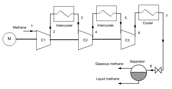
Methane liquefaction basic cycle
To liquefy natural gas methane taken at 1 bar and 280 K is compressed to 100 bar and then cooled to 210 K (it is assumed in this example that a refrigeration cycle is available for that).
Isentropic compression is assumed, but the very high compression ratio requires the use of several compressors (3 in this example) with intermediate cooling at 280 K. Intermediate pressures are equal to 5 and 25 bar.
The gas cooled at 210 K is isenthalpically expanded from 100 bar to 1 bar, and gas and liquid phases separated. As shown in the diagram in Figure below, the methane enters in the upper left, and liquid and gaseous fractions exit in the bottom right.
With the settings chosen, the synoptic view is given in Figure below.
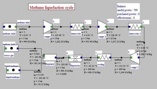
The compression work required per kilogram of methane sucked is 798.5 kJ, and 0.179 kg of liquid methane is produced, which corresponds to a work of 4.46 MJ per kilogram of liquefied methane.
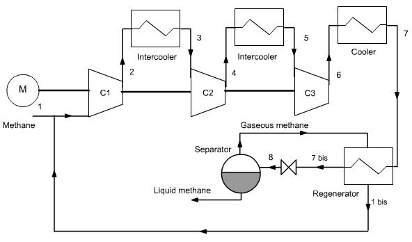
Linde cycle
The Linde cycle (Figure below) improves the previous on two points:
gaseous methane is recycled after isenthalpic expansion;
we introduce a heat exchanger between the gaseous methane and methane out of the cooler in order to cool the compressed gas not at 210 K but at 191 K.
For these new conditions the compression work per kilogram of liquefied methane becomes equal to 1.91 MJ, i.e. just 43% of the previous one.
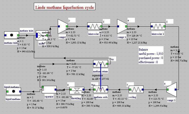
The calculation of this cycle requires some caution, given the sensitivity of the balance of the heat
exchanger to flow variations set by the separator.
The solution we found was to set the flow rate in the fi rst intercooler, then to recalculate the entire project by recalculating in addition the regenerator repeatedly. A stable solution could then be found, but it led to an inaccurate flow recirculation at the beginning. The correct rate value to set was obtained by successive iterations.
The performance gain comes mainly from the decrease of the expansion valve inlet temperature, which reduces the exit quality and thus increases the flow of the liquid phase. Moreover, the decrease in temperature at the inlet of the first compressor reduces the compressor work, but this effect is less important than the first.
Plot of the cycles in the thermodynamic charts
The plot of both cycles in (h, ln(P)) and entropy diagrams (Figures below) illustrates the benefits of the second: the leftward shift of point 7 in 7bis in the Linde cycle more than doubles liquid quality at the valve outlet (point 8).

Linde Cycle in red , and basic cycle in black
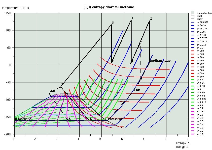
Linde Cycle in red , and basic cycle in black
Linde cycles for nitrogen liquefaction
As air is not modeled in Thermoptim as condensable, we will consider here the liquefaction of nitrogen.
Gaseous nitrogen at 1 bar and 280 K is compressed at 200 bar (cooled compression at 50°C), then cooled at 280 K.
Nitrogen is then cooled in a heat exchanger with the non-liquefied part, allowing it to reach a temperature of about -110°C. It is then isenthalpically expanded at 1 bar, thereby about 8% is liquefied.
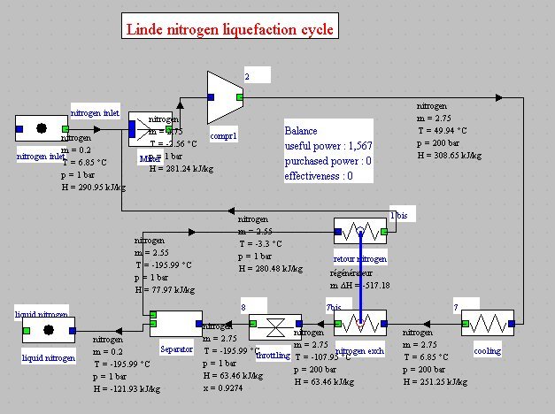
The liquid fraction is extracted, and the remainder in the form of saturated vapor is recycled in the regenerator and mixed with atmospheric nitrogen at 280 K, which closes the cycle. The performance of this machine is small, about 5.7 MJ/kg, but the cycle can be modeled without difficulty in Thermoptim (Figure below).
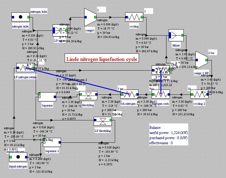
It can be improved by a double expansion cycle, but the setting is much more difficult to obtain because instabilities can occur in flow-rates, because of the role played by the phase separators (Figure below).
REVERSE BRAYTON CYCLE
The reverse Brayton cycle has been presented in a thematic page , which we recommend you to refer to for details.
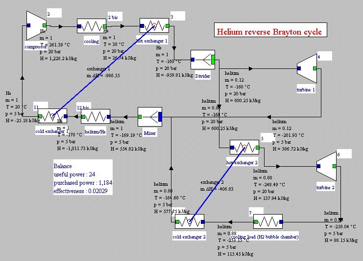
This cycle can be used for cryogenic applications. For example, Figure below shows the block diagram obtained for example 3.2.1 by B. Petit, relative to a plant for producing cooling below 20 K to refrigerate a liquid hydrogen bubble chamber.
In this cycle, helium is compressed to 20 bar, then cooled to 30°C before being divided into two streams which are expanded in parallel, the main stream following a conventional reverse Brayton cycle, while the secondary contributes to cooling the total flow.
Note that in this example, point 12a temperature must be set by hand, equal to that of point 12, because of the need to change the substance, the helium vapor being defined in Thermoptim only for T<200 K.
MIXED PROCESSES: CLAUDE CYCLE
The Linde cycle uses isenthalpic expansion which has two drawbacks: firstly the expansion work is lost, and secondly cooling cannot be achieved if the fluid thermodynamic state is such that the Joule Thomson expansion leads to a temperature lowering.
Claude has proposed a cycle that involves a turbine and an expansion valve and has the peculiarity that the plant operates with a single fluid compressed at a single pressure level, as shown in Figure below. The Claude cycle has been used in many air liquefying facilities.
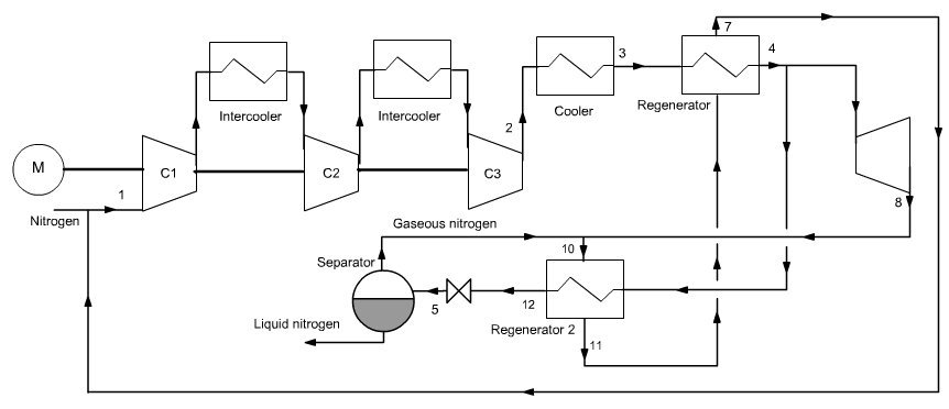
The advantage of this cycle is that the compression ratio can be significantly lower than in the case of the Linde cycle. One difficulty is that the expansion machine cannot operate with good efficiency if the fluid remains in the vapor zone or keeps a high quality. The originality of the Claude cycle is to combine isentropic expansion in the turbine, and isenthalpic expansion only in expansion leading to the gas liquefaction.
The beginning of the cycle is the same as that of Linde: compression of gas to liquefy, then cooling to about room temperature (1–3). The gas then passes through a regenerator which allows it to cool at about -105°C (3–4). The flow is then divided, about 15% being expanded in a turbine (4–8). The main flow passes through a second regenerator of which it is released at very low temperature (4–12). It undergoes isenthalpic expansion (12–5) and the liquid phase is extracted. The vapor is mixed with the flow exiting the turbine, and serves as a coolant in the second regenerator (10–11), then in the first (11–7) before being recycled by mixing with the gas entering the cycle.
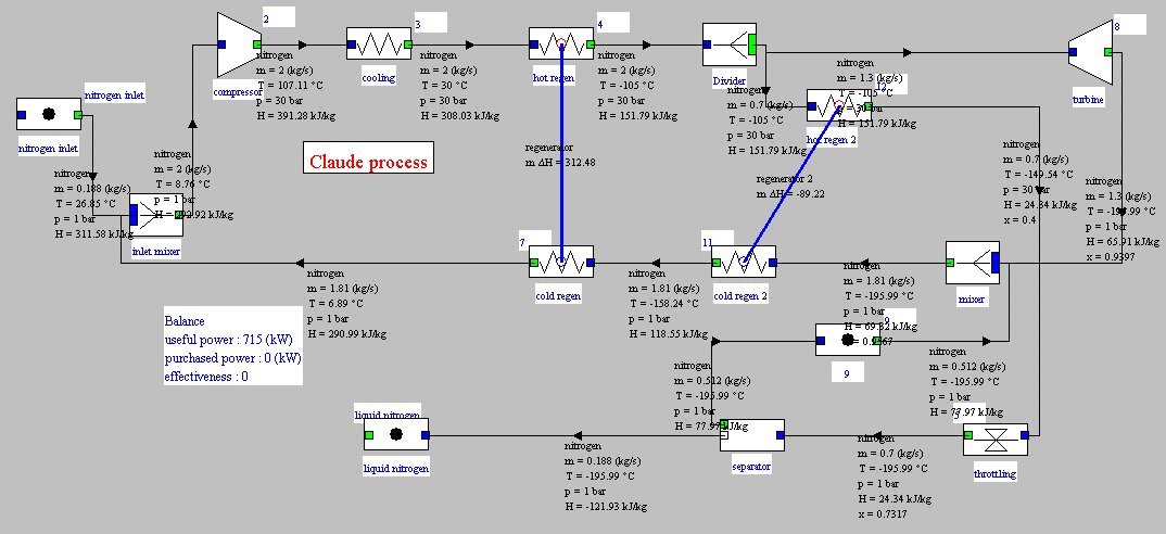
This cycle can be modeled with Thermoptim. Inspired by the example 3.2.2.2 by B. Petit presented in the Techniques de l'Ingénieur, we obtain the block diagram in Figure below. The compression power is about 3.8 MJ/kg.
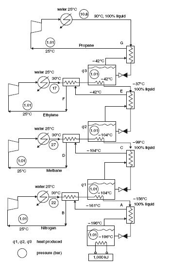
CASCADE CYCLES
It is also possible to use cascading refrigeration cycles, the evaporator of one of them serving as a condenser to another and so on (Figure below). The various cooling circuits are then independent from the hydraulic, but thermally coupled by their evaporative condensers.
An alternative, widely used nowadays in the liquefaction of natural gas, is to use a so-called incorporated cascade, using a single working fluid consisting of a mixture of methane, ethane, propane, butane and pentane.
Exercises and practical activities
As an exercise you can model the cycles presented above. Their correction will give you the corresponding Thermoptim files:
methane liquefaction
nitrogen liquefaction (Linde)
reverse Brayton helium cycle
nitrogen liquefaction (Claude)
References
ASHRAE, Cryogenics, ch. 38, Fundamentals Handbook (SI), 2002.
P. PETIT, Séparation et liquéfaction des gaz, Techniques de l'Ingénieur, J 3600.
S. SANDLER "Chemical and Engineering Thermodynamics" 3ème édition, J. Wiley editors, 1999
