This page provides some examples of the results that can be obtained when making technological design and off-design studies.

We refer the reader interested in more details to the presentation page of this issue and in Part 5 of the first edition of the book Energy Systems.

We will study the following examples:

• The design of an air-water exchanger;

• The determination of the displacement of an air compressor;

• The filling of a compressed air tank;

• The off-design operation of a refrigeration machine for producing brine at -10 ° C.

A link will be finally given to another example related to a steam power plant cycle.

You will find in the thematic pages explanations on heat exchangers and displacement compressors .

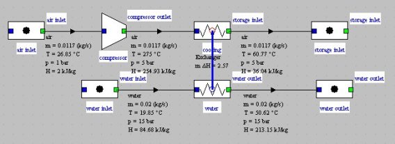
Let us consider a tube and fin heat exchanger cooling 0.66 kg/min (0.0117 kg/s) of air leaving a compressor at 5 bar and 275 °C with a flow rate of 1.17 kg/min (0.02 kg/s) of cold water passing through a coil of two parallel tubes. We neglect in this example the wall and fouling resistances. The thermal power transmitted is 2.57 kW.

The exchanger can be easily modeled in Thermoptim, leading to the screen shown above, and the synoptic view below.

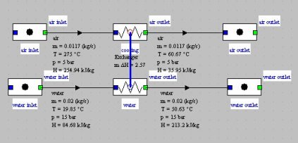
Synoptic view of a heat exchanger

To size the heat exchanger, we may set its effectiveness, for example equal to 0.84. Its screen is given below.

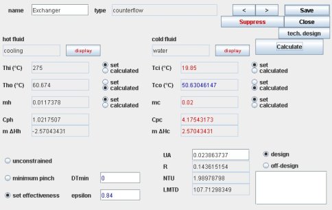
Classical exchanger screen

So far, we only used the classic features (phenomenological screens) of the package, and we do manage to get the UA product of the heat transfer coefficient by the surface of the exchanger, without being able to determine separately the values of each of these two factors. Here UA = 0.02386 kW/K, or 23.86 W/K).

Using the Thermoptim technological design screens, we can now calculate the overall heat transfer coefficient and deduce the area required to transmit the desired thermal load.

When you simply want to make the technological design of a project that implements components of the Thermoptim core, it is possible to automatically create technological screens using the generic driver, which avoids having to program one.

Open the Thermoptim project, and load the generic driver by choosing from among the list of drivers, the one which is labeled "generic techno design driver", then click "Set the technological design screens".

Warning: the generic driver requests that the diagram and the project are both loaded into Thermoptim.

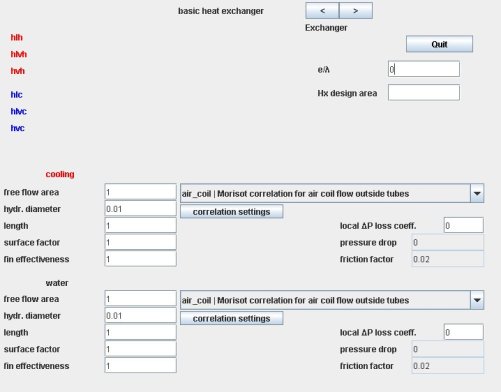
Exchanger default technological design screen

The technological design screen of the heat exchanger contains in the lower left part two areas, one for each "exchange" process.

In calculating the heat transfer coefficients and pressure drops, in addition to the surface of the exchanger, two parameters are still needed: the free flow area devoted to the fluid Ac, and the hydraulic diameter dh.

When, as is the case in this example, the heat exchange coefficients of the two fluids are very different, we use such devices as fins to compensate for the difference between their values. This is called extended surfaces, which can be characterized by a surface factor f and a fin efficiency eta.

These four parameters Ac, dh, f and eta are those that were selected to characterize the heat transfer in each fluid. The exchanger length is added for some calculations, including pressure drops.

• "free flow area" represents the section devoted to the fluid flow Ac;

• "hydr. diameter" is the usual hydraulic diameter dh;

• "length" is the length of the exchanger;

• "surface factor" is the surface factor f for extended surfaces;

• "fin efficiency" is the fin effectiveness eta;

• wall resistance e/lambda is entered in the top right of the screen under the "Quit" button. It allows one to take into account the fouling resistance if desired. In this example we neglect it.

The values of technological design parameters must be entered for both fluids, having chosen for each one the flow pattern in the list, here "ext_tube | Colburn correlation ..." for cooling air, and "int_tube | Mac Adams correlation ..." for water inside the tubes.

It is this flow configuration that specifies the correlations for the heat exchange and pressure drop coefficients that are used for the calculation of the exchanger.

We must first determine the hydraulic diameter dh and the free flow area Ac of the two fluids.

Inside the tubes, dh is given, and the calculation of Ac is very simple: it is equal to product of the number of tubes by the section of one of them. With an outside tube diameter of 15 mm and a thickness of 1.5 mm, inner diameter is 12 mm. A simple calculation shows that for two tubes, Ac is 0.000226195 m2.

Outside the tubes, the calculations are a bit more complicated. dh equals 4 times the wet perimeter.

Ac is the cross-sectional area available to the passage of air. We assumed that fins multiply by 4 the exchange surface, with an effectiveness equal to 0.8.

These values ​​must be entered in the heat exchanger technological design screen. By taking the parameters detailed in the breadcrumb trail on heat exchangers, we obtain the results shown in the figure below.

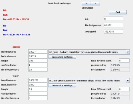
Set technological design screen

We can then calculate the required area A, which is here equal to 0.067 m2, the coefficients of exchange being worth 669 (W/m2/K) air side and 759 (W/m2/K) water side, as shown in the Figure, leading to an overall coefficient equal to 355.7 (W/m2/K).

The heat exchanger will be made up of two coil tubes each 90 cm long arranged on three layers crossing a total of 540 square iron plates of 2 cm side separated from each other by 3 mm.

If we want to be accurate, we enter this length value for the water side and 6 cm air side, allowing to refine the estimate of pressure drops.

Once the heat exchanger sized, its off-design behavior can be studied directly from the simulator screen.

The off-design calculation mode makes it possible to calculate the heat exchanger by the NTU method, considering that the two inlet temperatures and two flow rates are set.

Thermoptim performs an update of the exchanger links upstream of the processes, then calculates the outlet temperatures and balances it in terms of enthalpy, with the UA value entered in the screen field. Points and processes associated are updated based on the results.

However, no correction is made automatically on UA to account for the evolution of exchange coefficients based on flow rates and temperatures.

Make therefore a new calculation of the exchanger, estimate the value of the resulting U, and change UA accordingly, and then restart the calculation, by repeating the operation until values become stable.

All explanations related to this example are provided in the breadcrumb trail on heat exchangers .

When trying to size a displacement compressor, you first must determine its displacement so that it can transfer the desired gas flow. Thermodynamic calculations then lead to a value that usually does not correspond exactly to those proposed by the manufacturers. The machine chosen then differs slightly from that originally desired, so that the flow rate used differs from that which was wanted.

To represent the evolution of the volumetric efficiency as a function of the compression ratio, we can generally assume that it is linear, characterized by an intercept (or more precisely for a compression ratio equal to 1), and a negative slope.

To illustrate the type of design problem encountered, we will consider a diagram that will be used in the following example dealing with off-design behavior.

This is an air displacement compressor that fills a compressed air storage of given volume at variable pressure.

The compressed air is cooled before storage with a water exchanger of the type which has just been presented.

The system can be easily modeled in Thermoptim and leads to a diagram of the type of the figure below, which differs from that studied in the breadcrumb trail of heat exchangers by the addition of the compressor.

Synoptic view of the cooled air compressor

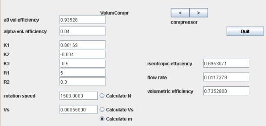
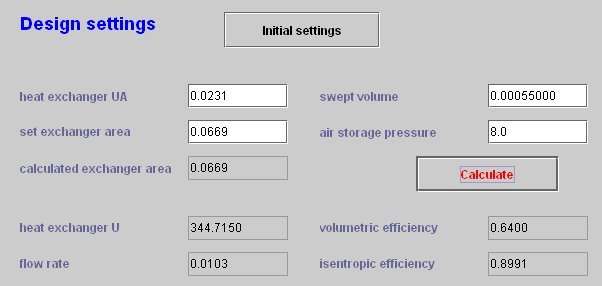
In this example, we assume that the compressor rotation speed is equal to 1500 rpm, and we seek what is the displacement required to compress from 1 to 5 bar the flow into play in the previous example, i.e. 0.01738 kg/s of air.

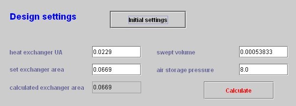
The screen of the driver used is presented in the following figure. By clicking "Initial settings", after checking "Calculate Vs" in the compressor TechnoDesign, so that Thermoptim knows that this value must be calculated, the required displacement is displayed in the field labeled "Vs" or 0.00055 m³, or 0,55 l.

A search in the catalog shows what is the closest available manufacturer's engine.

To change the model, the user then simply has to replace the displacement calculated by the new value.

Recalculation then leads to a rate be slightly different from that which was envisaged.

Determination of the displacement

To illustrate this type of calculation, we will now study the behavior of the air compressor, when used to fill a compressed air storage of given volume at variable pressure.

The model chosen for the compressor takes into account its volumetric and isentropic efficiencies as functions of the compression ratio. The first is given as we have seen by a simple affine relation, and the second has the shape of the figure below.

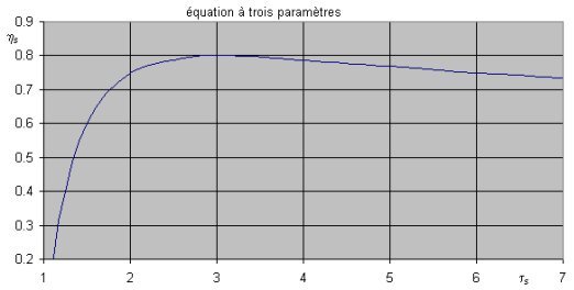
Compressor isentropic efficiency

The compressor technological design screen is given in the figure below. That of the exchanger is similar to the previous one.

Compressor technological screen

Role of the driver

To achieve the desired results, we must build a driver, whose screen may look like below. It allows us to vary the compression ratio to get the main value changes when the tank pressure varies, by operating as follows:

• Update the outlet compressor pressure

• Calculate the compressor volumetric efficiency

• Calculate the compressor isentropic efficiency

• Recalculate the compressor and downstream process

• Update the heat exchanger inlet and outlet points

• Determinate U, update UA and recalculate the heat exchanger in off-design mode (in various iterations since U depends on the average temperatures of the fluids, and therefore those of outlet points)

• Update the simulator and displays

Note that in this example the behavior of the compressor is independant, once the compression ratio set, of that of the downstream heat exchanger: there is no system coupling, at least for a given operating point .

The design of the driver is facilitated: there is no nonlinear coupling equation system to solve.

Cooled compressor driver screen

Once the driver made it very easy to vary the compression ratio for determining the main variables when the tank pressure varies.

Result files can be used with the Excel macro for post-processing Thermoptim simulation files presented in Volume 1 of the reference manual. Simply save the project files under a different name after each simulation, then load these files into the macro and extract the values of interest.

The figure below shows, depending on the storage pressure, changes in the compressor isentropic efficiency, compression work, intake air flow, temperature of air entering the tank, the exchanger load and UA.

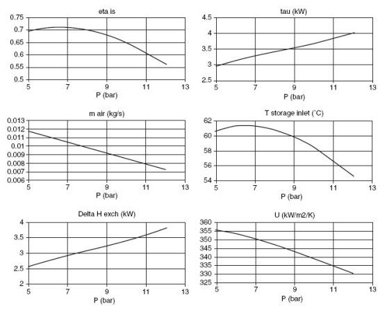
Influence of discharge pressure on the compressor performance

All the files for this example are given in the model library .

The results of the above figure can be used to simulate the filling of a compressed air storage. Thermoptim only providing results for steady state operation, the simplest is to develop a second model, solved with Excel.

Its equations are:

• the mass of air contained in storage M is equal to the initial mass plus the integral of flow;

• The internal energy U is equal to the initial internal energy plus the integral of the product of the flow by the air enthalpy leaving the cooler, less the integral of the loss by convection with ambient air;

• The storage temperature is inferred from its internal energy;

• The pressure is determined by the ideal gas law.

For the flow rate, the compression work and the temperature of the air entering storage, we have just to make polynomial regressions from simulations previously done with Thermoptim.

The look of the results is given figure below, for a storage of a half m3 (diameter 80 cm, length 1 m), powered by a compressor of displacement Vs = 0.525 l. The pressure and temperature in storage, its mass and the workload of the compressor are shown.

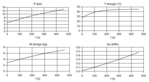
Filling of the compressed air storage

The files for this example are available for download in the model library.

We will now study a much more complex problem, that of the adaptation of a refrigeration machine to changes of the outside temperature or the compressor rotation speed.

So far we have discussed only relatively simple problems, which did not put into play systems of coupling equations between components. In this example, this is no longer the case:

• First, pressure levels are set by the thermal equilibrium of two phase-change heat exchangers, the evaporator and condenser, which set the saturation temperatures;

• The compressor sets the volumetric flow of refrigerant (depending on its rotation speed and compression ratio that determine its volumetric efficiency), and thus the mass flow rate (depending on the specific volume of refrigerant at the inlet).

The main parameters of the refrigeration machine, namely the pressure levels and flow-rate, are set by several components strongly coupled whose calculation cannot be done independently.

In addition, we set two additional constraints:

• we take into account the pressure drops in heat exchangers;

• sub-cooling is determined by ensuring the conservation of total mass of refrigerant contained in the machine.

Cycle setting

Suppose we want to size a simple refrigeration cycle (Figure below) to provide a cooling capacity of 130 kW for an outside temperature of 30 °C, the temperature of the brine being equal to -10 °C at the evaporator inlet.

For this cycle, the cold fluid is 40% by volume propylene glycol, available in the external substances. Evaporating temperature must of course be lower than that of the brine. We retained approximately -21.6 °C, that is to say a pressure of 1.24 bar for R134a.

We assume that the isentropic efficiency of the compressor is about 0.8 at design point. To simplify somewhat the model we assume that the value of the evaporation superheating remains constant (5 K). The condensation sub-cooling, however, is determined on the basis of the overall mass of refrigerant, which remains constant in the machine.

Evaporation superheating Tsurch is 5 K, which for a flow of refrigerant of 0.955 kg/s sets the cooling capacity at about 131 kW. With a brine flow of 15 kg/s, this leads to a cooling of 2.42 ° C.

For the condenser, the air temperature is 30 °C and its flow 25 kg/s. Condensing temperature is estimated at 42 °C, which, with an initial sub-cooling Delta Tssrefr of 5 K, corresponds to a condensation pressure of about 10.9 bar. The COP of the machine is 2.24 under these conditions.

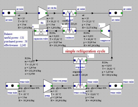
Synoptic view of the refrigeration cycle

Taking into account the refrigerant pressure drops takes some precautions to avoid difficulties in calculating the phases of condensation and evaporation. We chose to assign them only to points where the condition is single phase: in full downstream of the evaporator, and half upstream and downstream of the condenser.

The pressure drop on air and brine are calculated in the technological screens of exchangers and set as an over-pressure upstream of the exchanger. Fans and pump brine are here modeled by compression standard processes, without taking into account their detailed characteristics. It would be possible to do so, but at the cost of increased complexity that is not really justified.

The design is done in two distinct steps, the first one is the classic cycle setting in Thermoptim, while the second one is made from the technological screen. It should be noted, and this is very important, that the second step can be performed only when the first has been completed and has resulted in a fully consistent model. If this is not the case, the technological design made during the second step may be aberrant and cause great difficulties for convergence.

We will not detail here, for simplicity, how to build the cycle Thermoptim model corresponding to the first step. If it does not exist, you should build it first, then the method would be the same. This refrigeration cycle is similar to those presented in the Getting Started guides the software, the main difference being that the condenser is modeled by a single multi-zone heat exchanger, the desuperheater not being dissociated from the condensation itself in the diagram editor.

Driver screen

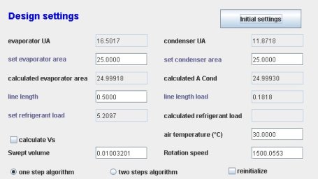
The upper part of the driver screen is given in the Figure below. It allows you to change on the one hand the exchanger surfaces, and also the length of the liquid line, air temperature, rotation speed or displacement, and has options for the algorithm guidance that will be specified later.

By default, the rotation speed is calculated for the value of the displacement entered in the screen. If you select "Calculate Vs" the displacement is calculated for the value of the speed entered.

Start by clicking "Initial settings" to instantiate the TechnoDesigns and make an initial technological design, in this case calculate the rotation speed or displacement of the compressor and the surfaces of the two exchangers corresponding to the project file setup, on the basis of default values for TechnoDesign parameters.

Driver screen (input parameters)

Technological screen setting

Once the technological screens have been created, you set them and size them. This must be done carefully because it involves making a series of choices about the internal configurations, the geometric dimensions...

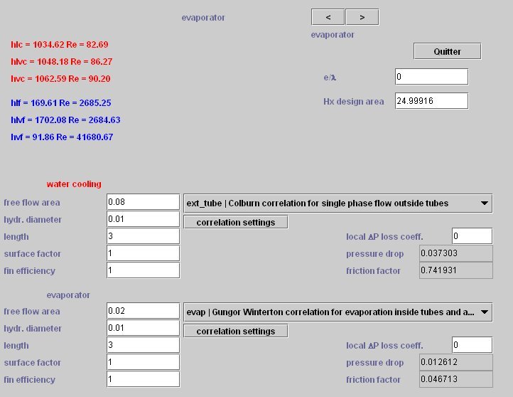
To access the technological screens, do so from the tables of the general simulator screen (Ctrl T) or from the "tech. design" buttons of component conventional screens.

We consider that the evaporator is of shell and tube type and has water side a fluid flow area of 8 dm2 and a hydraulic diameter of 1 cm, and refrigerant side a flow area of 2 dm2 and a hydraulic diameter of 1 cm, the tubing length being 3 m. Choose the type of configuration ("evap Gungor Winterton" for evaporation inside the tubes for the "evaporator" (refrigerant), and "ext tube Colburn correlation" for the brine, and set the screen as shown in the Figure below.

The condenser is of the finned coil type. Air side it has a fluid flow area of 1 m2 and a hydraulic diameter of 1 cm with an extended surface factor of 20, with a length of 15 cm (thickness of the air condenser), and refrigerant side a fluid flow area of 0.5 dm2 and a hydraulic diameter of 2 cm, the tubing length being 3 m.

Choose the type of configuration ("cond Shah correlation" for condensation inside the tubes for the "condenser" (refrigerant), and "air coil Morizot correlation" for air, and set the screen as shown in the Figure below.

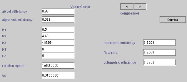
For the compressor (Figure below), we must provide first the displacement Vs, and secondly the values of the parameters involved in the equations of isentropic and volumetric efficiency.

To achieve the technological design once the screens filled, click again on the "Initial settings" screen of the driver.

The results are displayed in the technological screen: exchange surfaces of 25 m2 for the evaporator and condenser; rotation speed of 1500 rpm and displacement of about 0.01 m3 for the compressor.

Various calculation results are displayed on the technological screen, such as, for heat exchangers, pressure drop and the values of the Reynolds number Re and the local exchange coefficients.

Resolution of the off-design system of equations of the refrigeration machine

In any study of off-design behavior, we must identify what are the independent variables of the system considered, distinguishing them from variables that are deduced.

In this example, it is the quadruple (refrigerant flow, evaporating temperature, condensing temperature, sub-cooling), the variables being the fluid pressures and the thermal and mechanical capacities. To these four "natural" variables must be added the two intermediate variables UAevap and UAcond. which make it possible to ensure the calculation of the heat exchangers, the convergence criterion being that their surfaces remain equal to those of design

The search for this sextuplet corresponds to the solution of a set of relatively complex nonlinear equations.

The solution we have adopted is to build an external driver that provides the resolution of this system of equations and updates Thermoptim once the solution found.

We use the Marquardt Levendberg method implemented in algorithms developed in Fortran as the minPack 1 package, and translated in Java. This method combines the Gauss-Newton method and gradient descent. Its main interest is to be very robust and to only require as initialization an approximate solution.

Its implementation in Java is done using an interface called optimization.Lmdif_fcn, which forces the calling class (in this case our driver) to have a function called fcn() that returns the difference, called residual, between the target value and the calculated value.

Guiding the algorithm is done by playing on two criteria of accuracy, one on the sum of the residues, and the other on the accuracy of the partial derivatives, estimated by finite differences. Remember that we are trying to solve a system of six nonlinear equations in six unknowns, which can be numerically difficult. In practice, it was interesting to propose several options for calculating.

First, the "Reinitialize" option offers the ability to reset the evaporation and condensation temperature values according to those of the brine and the ambient air, to avoid temperature crossing in exchangers.

Then, two exclusive options are available: either run the algorithm in one step, for intermediate values of accuracy of the convergence criteria ("one-step algorithm"), or run it in two steps, first to a coarse convergence and the second more accurate ("two steps algorithm").

You can choose one or the other, depending on the numerical difficulties encountered. An indicator of accuracy, corresponding to the L2 norm of residuals, is shown in the result part of the driver screen (Figure 6).

If you start calculations from the General screen of technological screens, you can furthermore, if you wish, interrupt the calculations properly by clicking the "Stop" button, which allows you to change options. Be careful, because this way of working can lead to errors.

Simulation results

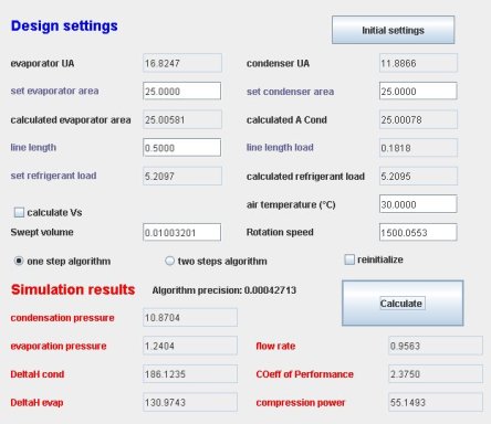
The full screen of the driver is given in the Figure above. It allows you to change the exchanger surfaces and the length of the liquid line, as well as the air temperature, displacement or rotation speed.

Enter the air temperature or the speed you want to change, and either click "Calculate" or open the TechnoDesign screen from the simulator, then click "Calculate the driver." The second way is preferable because it allows you to track the convergence while keeping hands on Thermoptim to display intermediate values or modify the calculation of the driver.

The results are displayed on the screen once the convergence obtained. If the values you enter are very different from those of design, Thermoptim calculation errors can be generated with messages. If necessary, choose a target value closer to the initial value.

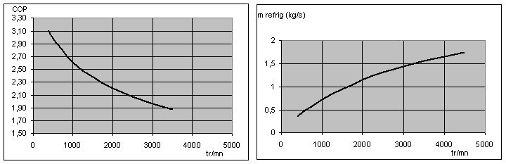
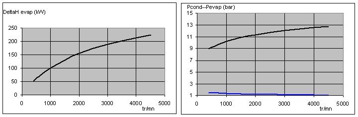
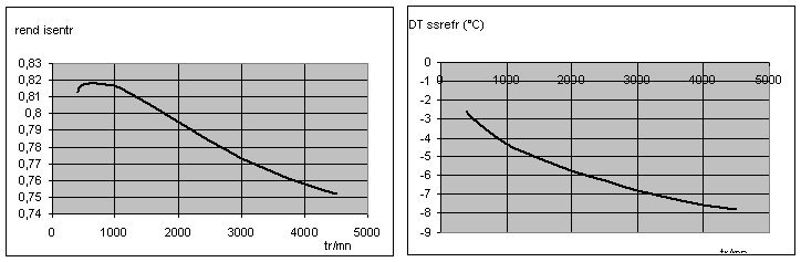
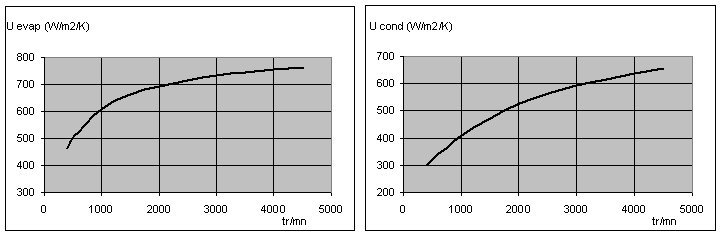
The figures below show the simulation results obtained when we vary the temperature of the cooling air, for the setting of technological screens previously selected, the speed being equal to 1,500 rpm. They clearly show the nonlinearity of the behavior of the machine.

Note that the heat exchange coefficients vary significantly, which fully justifies that we do not consider them constant.

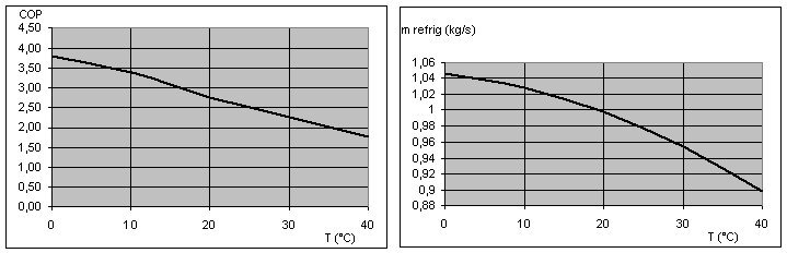
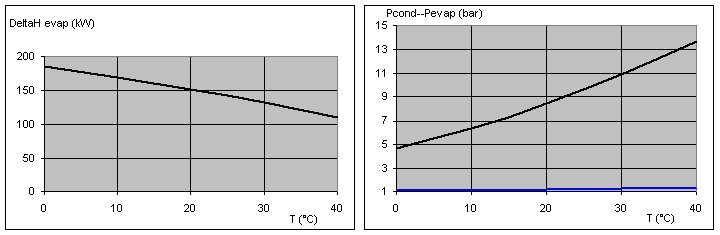
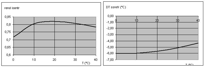
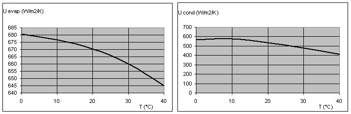
The influence of the rotation speed is given in the figures below, for an outside temperature of 30 ° C.

In this example, we have varied only two variables, but it would be easy to study the influence of air and brine flows, or temperature of the latter, either by modifying their values in the simulator screens before recalculation with this driver, or by modifying it so that these values appear in the driver screen so that they can be automatically updated.

All the files for this example are given in the model library.

A similar example was built to explain how to create a driver allowing one to study the off-design behavior of a steam power plant. It is also available in the model library . Since it is very similar to the example we just presented, we do not develop here.

It should be noted that in-depth studies were carried out in 2021 on the correlations relating to pressure drops and heat exchange coefficients used since 2009, in order to take into account the numerous results published over the last twelve years.

Some approximations that were initially made to reduce computational times were questioned on this occasion, as current processors are much faster than at the time.

Some errors were also detected and corrected, and some models were completed. Therefore, the results provided by the late 2021 versions show some differences with those of 2009 presented above. They relate essentially to the values of the calculated areas, the rates of evolution in off-design regime remaining similar.

The main discrepancies found are explained in the pages of the model library providing the files of these examples.

A document explaining how to practically use the driver built for calculating the off-design operation of a refrigeration machine can be downloaded from the link below, as well as result files and Excel spreadsheets for this refrigeration machine and the simplified steam power plant mentioned above.

The versions of Thermoptim that allow one to make technological design and off-design studies are versions 2.7 and 2.8.