In this educational breadcrumb on heat exchangers, we will start by briefly recalling what such components are and giving some elements of theory on how they can be calculated. We then detail the analysis and design of a heat exchanger allowing one to cool the air exiting a compressor.

This is an example intended to diagnose the problems and show how they can be resolved without the overall system being too complicated. For specialists, it will seem a bit simplistic, but for beginners it is already quite difficult to treat completely.

It uses Thermoptim versions 1.7 or 2.7 currently under development.

The mind map below summarizes the main concepts to be discussed here

In functional terms, the heat exchangers are devices used to transfer heat between two fluids at different temperatures.

An example of fairly well-known heat exchanger is the "radiator" of an automobile, which allows one to cool the engine by rejecting excess heat in the atmosphere. It prevents motor damage due to overheating of the mechanical parts. In case of failure of this component, a serious accident such as blocking of the engine by "pouring" rod can occur.

Technologically, although there is a very large variety of heat exchanger models, the four main categories used in energy systems are:

• Tubular exchangers

• Shell and tube exchangers

• Air coils

• Plate heat exchangers

Generally, the two fluids are not in contact, and the transfer takes place through an exchange area. Within the dividing wall, the heat transfer mechanism is conduction, and on each of both surfaces in contact with fluids, convection almost always predominates.

In many cases, fluids are single phase, whether gas or liquid. However, there are three main types of heat exchangers in which phase changes occur: the vaporizers or evaporators where it vaporizes a liquid, the condensers where steam is liquefied and evaporative condensers where both fluids change phase. We limit ourselves to single-phase exchangers.

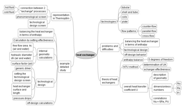
The diagram below will clarify the notations that we use. We will denote the hot fluid by index h, and the cold fluid by index c. Besides the geometric configuration, exchanger design or performance depends on many parameters and variables:

• mass flows mc and mf passing through them;

• inlet temperatures Thi and Tci and outlet temperatures Tho and Tco of both fluids.

In practice, heat exchangers are of great importance in many energy systems in which heat is transferred, especially when attempting to recover thermal energy.

They can play a critical role in the performance of energy systems involving internal heat exchange, such as regeneration or combined cycles, whose optimization requires one to minimize the internal irreversibilities related to internal temperature differences.

The study of heat exchangers in an energy system can be done at very different levels of difficulty depending on the objectives that we pursue:

The most basic approach, very simple to implement, is to balance the heat exchanger in terms of enthalpy by determining for example the outlet temperature of a fluid when the inlet temperatures and flow rates of the two fluids are known, as well as an outlet temperature;

The problem can be posed in reverse, if the two outlet temperatures are known and only one inlet. The approach remains simple.

One can indeed show that a heat exchanger has five degrees of freedom and once five are set among the input and output temperatures and flow-rates, the sixth is directly deduced;

It is also customary to characterize a heat exchanger by an effectiveness or by a minimum temperature difference between the two fluids (called a pinch). Solving this problem is also quite simple if four other quantities are known.

We call this type of study elementary calculations balancing the exchanger enthalpy.

Note that, very often in the study of energy systems, heat exchanger calculations are not explored further. They indeed already provide sufficient information to conduct preliminary analysis of many cycles, especially at the functional level, apart from specific technological considerations.

The theory shows, as we see in this chapter, that this approach allows us to characterize an exchanger by what we call the UA, the product of the internal heat exchange coefficient between the two fluids U by its exchange area A.

To go further and determine the exchange surface required, calculations are much more complicated, requiring a thorough knowledge of the inner operation of heat exchangers, in order to estimate as precisely as possible the value of U. There is actually a very important qualitative leap between the basic arithmetic of balancing the heat exchanger and what we call its technological design.

This is by the way a general problem in energy systems studies: as long as one is satisfied to carry out cycle studies without trying to size the geometry of the components, the calculations are much simpler than when one wishes to closely analyze their internal behavior.

Once the surface of a heat exchanger determined, which allows one to characterize it geometrically plan, another problem remains to be treated: that of his behavior when operating conditions differ from those used for the design. How does the exchanger fit to changes in flow rates and inlet temperatures of fluid passing through it?

We call this problem to study its off-design behavior.

It can be a higher level of complexity than the technological design, because it may require solving large systems of nonlinear equations when several components are coupled together.

Given the objective of the educational breadcrumb, which is to provide a guide to help teachers and students understand how concepts are linked, we will simply indicate the key milestones on the theory of heat exchangers, referring the reader to the thematic page on the subject, and also to literature.

Three assumptions are generally used to model a heat exchanger:

• At first approximation, it can be considered as isobaric (specifically, pressure drops are low);

• It is globally adiabatic, that is to say that there is no heat exchange with the surroundings;

• Heat transfer coefficients and thermophysical properties of fluids maintain a constant value at any time in the whole of the heat exchanger (this assumption is not included in Thermoptim, where these properties are temperature dependent and thus vary between the inlet and outlet of the exchanger).

In general, the design of heat exchangers is a compromise between conflicting objectives, whose two main ones are:

• a large exchange area is desirable to increase the effectiveness of heat exchangers, but it results in high costs;

• small fluid flow sections increase the values of the heat exchange coefficients, and thus reduce the area, but they also increase pressure drops.

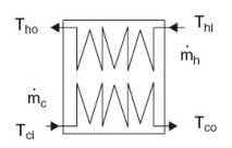
The heat flux exchanged can be expressed in three main equivalent ways, depending on whether the expression is referred to the hot fluid, the cold fluid or both fluids:

The first two equations express the heat lost by the hot fluid and received by the cold fluid, while the third expresses this flow as proportional to the heat transfer coefficient U, the surface of the heat exchanger A and the average temperature between the two fluids, called the logarithmic mean temperature difference .

Indeed, as the temperature varies along the heat exchanger, a simple medium value is not sufficient to determine the average difference in temperature between the two fluids: the value to be considered is given by the last equation above where and are the differences in fluid temperatures respectively at respectively at one end and at the other end of the exchanger, with the convention: .

Traditionally, the design of heat exchangers has long been using the logarithmic mean temperature difference method, but it is not always easy to implement.

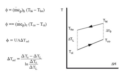
The calculation method we advocate is that of the NTU, or number of transfer units, developed more recently and easier to use in practice. We content ourselves here with a very concise presentation, referring the reader interested in further developments to the first edition of the bookEnergy Systems.

By definition, NTU is defined as the ratio of the product UA of the heat exchanger to the minimum heat capacity rate:

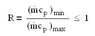
We call R the ratio (less than 1) of the heat capacity rates:

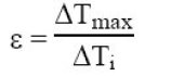
 is the difference between inlet temperatures of both fluids, and l

the maximum temperature difference within each of the two fluids and not between them.

We call e the efficiency of the exchanger, defined as the ratio of to :

With these definitions, it is possible to show that there is a general relation of type:

= f(NTU, R, flow pattern)

In a heat exchanger, the fluid flows can be performed in multiple arrangements: counter-flow, parallel-flow, cross-flow.

One can easily show that thermodynamically, the most efficient heat exchanger is the counter-flow heat exchanger, but other concerns than the thermodynamic effectiveness are taken into account when designing a heat exchanger: the maximum permissible temperatures in one fluid, or more often considerations of size, weight or cost.

In this simplified presentation, calculations will be made with the counter-flow configuration, even if the example treated is cross-flow. The error remains small.

In practice, it suffices to have a set of relationships corresponding to flow patterns representative of exchangers studied, and the design of a heat exchanger is made on the basis on the one hand of the balance equations and on the other hand of these relations.

In design mode, knowing the flow-rates of both fluids, their inlet temperatures and the heat flux transferred, the procedure is as follows:

• we start by determining the outlet temperatures of fluids from the balance equation;

• we deduce the fluid heat capacity rate m cp of fluids and their ratio R;

• the effectiveness is calculated from and ;

• the value of NTU is determined from the appropriate (NTU, ) relationship;

• UA is calculated from the equation defining NTU.

In off-design mode,if you know UA, the equation defining NTU gives its value, and you can determine ) from the appropriate (NTU, ) relationship. The balance equation allows you to calculate the heat transferred

The NTU method, used in the Thermoptim phenomenological version, provides only the product UA of the global exchange coefficient by the surface of the exchanger, without the two terms being evaluated separately.

To size the heat exchanger, i.e. calculate its surface, one must on the one hand choose its geometry, and secondly calculate the overall exchange coefficient U, which depends on the configuration and fluid thermophysical properties

The overall heat transfer coefficient U depends on the distribution of thermal resistances in the exchanger. If the exchange surfaces are equal for both fluids, its value is given by the equation below, where e / l is the thermal resistance of wall of thickness e, l being the conductivity of the material:

The values of convection coefficients hh and hc are based on fluid thermophysical properties and exchange configurations, convective regimes being strongly dependent on the flow velocity.

Their determination relies on fluid mechanics and convection thermal engineering, including turbulent.

Putting them into equations leads to very complex representations that have generally no analytic solution. Given this difficulty, it is customary to use the possible similarity laws to obtain reasonably accurate results.

Without going into details beyond the scope of this presentation, the similarity laws state that the heat exchange between a fluid and a wall can be characterized by several dimensionless numbers called:

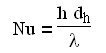
• Nusselt number Nu;

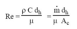
• Reynolds number Re;

• and Prandtl number Pr.

The expression for the Nusselt number is as follows, lambda being the conductivity of the fluid and dh the hydraulic diameter:

Re is usually defined in terms of the density , the flow velocity C, the hydraulic diameter dh and the kinematic viscosity .

By showing the free flow area devoted to the fluid Ac, it can also be expressed in terms of mass flow, hydraulic diameter dh and kinematic viscosity .

Pr depends on the kinematic viscosity , the heat capacity cp and the conductivity of the fluid , that is to say, its solethermophysical properties.

The laws of similarity establish that the Nusselt number is a function of Reynolds and Prandtl numbers.

The Nusselt number is almost always given by the following equation where C1, a, b, and c are constants:

The viscosity correction is made at the wall temperature. Coefficients C1, a and b vary depending on configurations encountered, and the additional term to account for variations in viscosity is often neglected.

In general, the Reynolds number exponent is between 0.5 and 0.8, and that of the Prandtl number between 0.33 and 0.4.

Such correlations, whose existence is validated by the theory, are in practice identified experimentally by performing a large number of tests with many fluids for varying hydraulic diameters, speeds and different heat fluxes. ..

Regressions are then digitally performed to identify the parameters of formulas of the type above.

The flow regime has a significant influence on the value of Nu. Where Re is less than 2,000, the regime is laminar, and if Re is greater than 5,000, it is turbulent, with a transition zone, these boundaries not being perfectly stable.

turbulence helps the heat exchange, but its counterpart is an elevation of pressure drops.

A specific page of this portal is dedicated to the presentation of the correlations that have been implemented in the external classes of Thermoptim to allow the study of the design of heat exchangers and their behavior in off-design behavior.

Let us recall that an "exchange" process is used to calculate the heating or cooling of a fluid between two states represented by upstream and downstream points.

It is symbolized in Thermoptim by the icon:

In Thermoptim, a heat exchanger is not represented by a particular component, but by a connection established between two "exchange" processes representing the hot and the cold fluids.

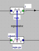
To represent the heat exchanger in the diagram editor, we use non-oriented links connecting two components of type "exchange".

Given the assumptions, the heat exchanger is necessarily balanced in terms of enthalpy, that is to say that the enthalpy transferred by the hot fluid is exactly equal to that received by the cold fluid.

Since there are four temperatures (two for each fluid) and two flow rates, the problem has five degrees of freedom once the enthalpy is conserved. One can furthermore show that at least one of the two flow rates has to be set, otherwise the problem is indeterminable.

Thermoptim proposes multiple design options for these degrees of freedom.

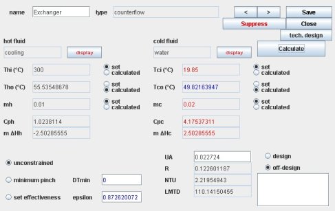
The figure above shows the screen of a heat exchanger in Thermoptim. It contains information about the hot fluid in the middle left part, while that for the cold fluid is in the right part.

Besides the values of temperatures, flow rates, heat capacities and enthalpies involved, constraints exist on the temperatures and flow rates used to manage the heat exchanger calculations, allowing one to distinguish between the variables of the problem, those set and those to be calculated.

In the bottom left, there are three buttons to optionally specify the absence or presence of implicit constraints on temperatures.

In the lower right are placed options for defining the calculation method ("design" or "off-design").

The design results of the heat exchanger are displayed in the fields at the bottom center of the screen, providing the values of UA, R, NTU and LMTD. The UA field is editable, allowing as we shall see to change it to perform off-design calculations.

Enthalpy balance

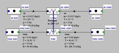
Let us consider a tube and fin heat exchanger cooling at 75 °C approximately 0.66 kg/min (0.0117 kg/s) of air leaving a compressor at 5 bar and 275 °C with a flow rate of 1.17 kg/min (0.02 kg/s) of cold water passing through a coil of two parallel tubes.

The heat flux to be removed is equal to about 2.4 kilowatts: 0.011738 . 1.022 (275-75), which leads to heating of the water close to 28.75 ° C: 2.4/0.02/4.1753.

The exchanger can be easily modeled in Thermoptim, leading to the screen shown above, and the synoptic view below.

Calculation by setting the effectiveness

To size the heat exchanger, it is common to set the effectiveness, for example equal to 0.84 instead of the previously determined value of 0.78. The synoptic view of the heat exchanger is given below: the thermal capacity is significantly increased.

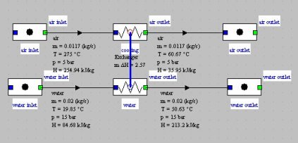
Synoptic view for a heat exchanger effectiveness equal to 0.84.

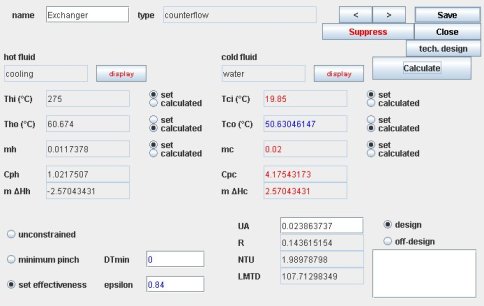
The main sizes and dimensions are calculated and displayed at the bottom of the screen:

• UA is 0.02386;

• R, ratio of heat capacity rates, is 0.1436;

• NTU, the number of transfer units is equal to about 2;

• LMTD, logarithmic mean temperature difference, is 107.7 °C.

So far, we only used the classic features (phenomenological screens) of the package, and we do manage to get the UA product of the heat transfer coefficient by the surface of the exchanger, without being able to determine separately the values of each of these two factors. Here UA = 0.02386 kilowatts/K, or 23.86 W/K).

We will now show how it is possible to refine our analysis.

Internal geometric calculations

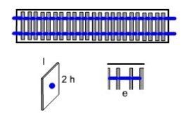
Suppose our exchanger consists of tubes and fins, the cold water passing through a coil made of several passes of two tubes in parallel as shown in the figure below where they appear horizontally in blue. The tube diameter is 15 mm, and its thickness 1.5 mm. Fins, represented vertically and gray, are crimped around the perpendicular tubes. The spacing e between the fins is 3 mm, their half-height h of 1 cm, their depth 2 cm and their thickness 0.3 mm.

In calculating the heat transfer coefficients and pressure drops, in addition to the surface of the exchanger, two sizes are still needed: the free flow area devoted to the fluid Ac, and the hydraulic diameter dh.

When, as is the case in this example, the coefficients of heat exchange of the two fluids are very different, we use such devices as fins to compensate for the difference between their values. This is called extended surfaces, which can be characterized by a surface factor f and a fin efficiency eta.

Inside the tubes, dh is given, and the calculation of Ac is very simple: it is equal to product of the number of tubes by the section of one of them. With an outside diameter tubes of 15 mm and a thickness of 1.5 mm, inner diameter is 12 mm. A simple calculation shows that for two tubes, Ac is 0.000226195 m2.

Outside the tubes, the calculations are a bit more complicated. One of the quantities to be determined is the number of fins Nf, and the other the overall number of passes. They cannot be determined by iteration, including the first, which directly influences the free flow area devoted to the air.

To avoid long explanations, we will retain immediately the result obtained, namely 90 fins.

Determination of free flow area for air

The flow area per tube is equal to:

AC0 = (2 h - d) e = 0.000015 m2

The number of tubes being equal to 2, the overall free flow area is:

Ac = 0.0027 m2

Determination of the hydraulic diameter for air

The wetted perimeter is:

p = 2 (2 h + e) = 0.046 m

This allows one to calculate the external hydraulic diameter:

Ac = dh 4 / 4 p = 0.001304348 m

Determination of the air surface factor

We must first calculate the initial surface of the tube or pi d e:

S = 0.000141372 m2

and the extended surface that is, by fin:

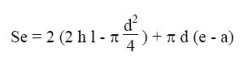
Se = 0.000573805 m2

We deduce the surface factor, ratio of these two values,:

f = 4

The fin efficiency will not be calculated here, but simply estimated equal to 0.8.

In addition, the length of the exchanger is:

Le = Nf (e + a) = 0.297 m

Using the Thermoptim technological design screens, we can now calculate the overall heat transfer coefficient and deduce the area required to transmit the desired thermal load.

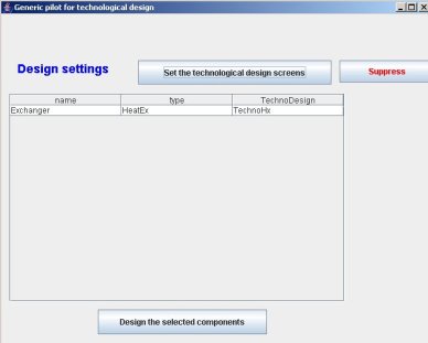
When you simply want to make the technological design of a project that implements components of the Thermoptim core, it is possible to automatically create technological screens using the generic driver, which avoids having to program one.

Open the Thermoptim project, and load the generic driver by choosing from among the list of drivers, the one whose title is "generic techno design driver", then click "Set the technological design screens".

Warning: the generic driver requests that the diagram and the project are both loaded into Thermoptim.

A line appears corresponding to the heat exchanger, as in Figure below. Select it.

Its type is by default HeatEx, and its TechnoDesign technoHx. Since it is a simple heat exchanger, they are perfect. Double-clicking on this line would change the type of TechnoDesign, but this is not necessary.

To display the technological design screen, the simplest here is to open the exchanger and click on "tech. design" located just above the "Calculate" button.

The default technological design screen is displayed as shown below. We will now see how to set it.

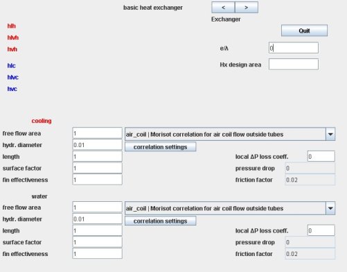
Exchanger default technological design screen

The technological design screen of the heat exchanger contains in the lower left two areas for each "exchange" process.

It includes, for each of the two fluids, the four parameters Ac, dh, f and eta. They exchanger length is added for some calculations, including pressure drops.

• "free flow area" represents the section devoted to the fluid flow Ac;

• "hydr. diameter" is the usual hydraulic diameter dh;

• "length" is the length of the exchanger;

• "surface factor" is the surface factor f for extended surfaces;

• "fin efficiency" is the fin effectiveness eta;

• wall resistance e/lambda is entered in the top right of the screen under the "Quit" button. It allows one to take into account the fouling resistance if desired. In this example we neglect i.

The values of technological design parameters must be entered for both fluids, having chosen for each one the flow pattern in the list, here "ext_tube | Colburn correlation ..." for cooling air, and "int_tube | Mac Adams correlation ..." for water inside the tubes.

The values that were determined above must be entered in the technological design screen of the heat exchanger. For now, the lengths of the heat exchanger are not known, since the number of passes is not determined. Ultimately, we will see that it is equal to 3. The values entered in the screen below correspond to this.

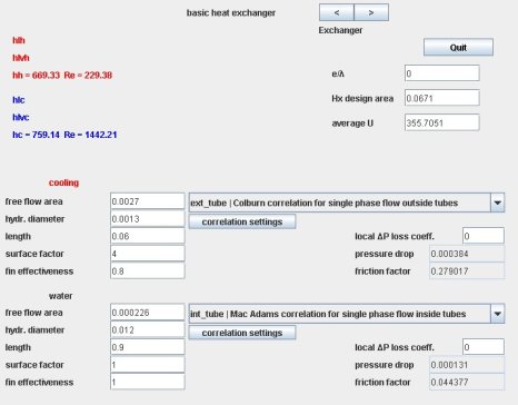
Set technological design screen

Once the settings done, return to the generic driver screen, then click "Design the selected components".

The results are displayed in the technological screen: the exchange surface needed is here equal to 0.067 m2, the exchange coefficients being worth 669 W/m2/K air side and 759 W/m2/K water side.

The number of passes can be deduced from these results. It is the ratio of the surface of the heat exchanger to the inner surface of the two water tubes, close to 3 in view of the selected geometry values.

We said above that the number of passes and number of fins could be found by iteration. Indeed, the first being an integer, and the second sets the free flow area devoted to air. You may therefore need to test several sets of values before a finding one that is consistent.

The lengths to be considered for the calculation of pressure drops can be determined now: 3 Le = 90 cm for the tubes (ignoring the elbows between the layers) and 3 l = 6 cm for the fins.

The heat exchanger will be made up of two coil tubes each 90 cm long arranged on three layers crossing a total of 540 square iron plates of 2 cm side separated from each other by 3 mm.

The pressure drop values (in bar) appear on the right side of the screen. They are negligible in our case.

The files for this example are available for download .

Off-design calculations

In off-design mode, we generally know the inlet temperatures and flow rates of fluids through the exchanger. An initial estimate of U can be performed, even if it can be refined when the outlet temperatures are known.

The exchange surface being known, the UA product can be determined, which gives the value of NTU.

We can then calculate e from the appropriate relationship (NTU, e).

One of the two outlet temperatures is obtained from the definition of e and the enthalpy balance provides another.

In practical terms, there are two main ways of operating:

• either by changing the UA and recalculating the heat exchanger in off-design;

• or directly by recalculating the NTU and epsilon, in particular if the inlet conditions can be changed. This is particularly the case of two-phase heat exchangers, whose thermal equilibrium establishes the change of state temperature and thus the pressure, which has the effect of changing both the inlet and outlet conditions.

The first way, the simplest is to use the off-design calculation mode of the exchanger screen. This can be done directly by hand, entering the new value of UA in the corresponding field, or by programming.

Once the heat exchanger sized, its off-design behavior can be studied directly from the simulator screen.

The off-design calculation mode makes it possible to calculate the heat exchanger by the NTU method, considering that the two inlet temperatures and two flow rates are set.

Thermoptim performs an update of the exchanger upstream links from the processes, then calculates the outlet temperatures and balances it in terms of enthalpy, with the UA value entered in the screen field. Points and processes associated are updated based on the results.

However, no correction is made automatically on UA to account for the evolution of exchange coefficients based on flow rates and temperatures.

Make therefore a new calculation of the exchanger, estimate the value of the resulting U, and change UA accordingly, and then restart the calculation, by repeating the operation until values become stable.

For example, look at how would behave the exchanger if the flow and temperature of the incoming air were changed, rising from 0.01174 to 0.1 kg/s and 275 to 300 ° C.

Proceed as follows:

1. modify in Thermoptim the exchanger inlet conditions, choose " off-design " in the heat exchanger screen;

2. recalculate several times the heat exchanger, until getting stable values;

3. finally, click button "Design the selected component" of the the generic driver screen.

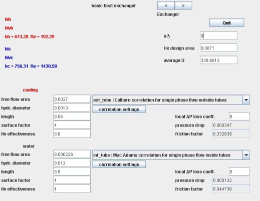
The new value of U is calculated: it is 338.7 kW/m2/K.

Multiplying this value by the exchanger surface, you get a new value of UA, equal to 0.022725, that you enter in the corresponding heat exchanger screen field.

Repeat steps 1 to 3: a more accurate estimate of U is obtained, taking into account the new setting. It is 338.66 kW/m2/K.

Amend UA accordingly again, which provides exchanger and TechnoDesign screens below.

The error we would commit on the estimation of UA by assuming it to be constant is here around 5%.

The exchange surface is the same as defined at the design.

Above, we manually changed the value of UA in the exchanger, the technological screen being built by the generic driver. This way of working has the advantage that it requires no programming, but it is a bit long to put into practice when several iterations must be performed. It would become tedious if it were to simulate the off-design behavior of the heat exchanger for a wide range of variation of operating conditions.

In this case, it is far better to automate these updates using a specific driver. One such example is shown in the breadcrumb trail on positive displacement compressors