Educational breadcrumb on on positive displacement compressors
Presentation
In this educational breadcrumb on on positive displacement compressors, we will start by briefly recalling what such components are and giving some elements of theory on how they can be calculated. We then detail the analysis and design of a piston compressor used to supply a storage tank of compressed air.
This is an example intended to diagnose the problems and show how they can be resolved without the overall system being too complicated. For specialists, it will seem a bit simplistic, but for beginners it is already quite difficult to treat completely.
It uses Thermoptim versions 1.7 or 2.7 currently under development.
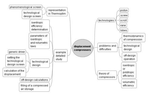
The mind map below summarizes the main concepts to be discussed here:
What is a compressor?
In functional terms, the compressors are devices used to increase the pressure of fluid passing through them.
Compressors are used for many industrial applications, refrigeration, air conditioning, transportation of natural gas...
Special mention should be made of air compressors, used as a source of power in public works and construction and in factories, pneumatic tools having many benefits. The example presented here focuses on this type of device.
Technologically, compressors can be grouped into two broad classes:
Positive displacement compressors, in which the fluid is trapped in a closed volume which is reduced gradually to achieve compression;
And dynamic compressors, which use a different principle: the compression is obtained by converting pressure into kinetic energy imparted to the fluid by moving blades.
We will limit ourselves in what follows to the study of positive displacement compressors, of which there are generally:
the piston compressors
the screw compressors
the scroll compressors
the vane compressors
the lobe compressors
A displacement compressor is characterized by encapsulation of the flow passing through it in a closed volume which is gradually reduced. A return of this fluid in the direction of decreasing pressure is prevented by the presence of one or more movable walls. In this type of machine, the kinetic energy imparted to the fluid usually does not play any useful role, unlike that which happens in turbomachinery.
By design, the displacement compressors are particularly suitable for processing relatively low fluid flow rates, possibly highly variable, and under relatively high pressure ratios..
Their operating principle is: a fixed mass of gas at suction pressure P1 is trapped in a chamber of variable volume. To increase pressure, the volume is gradually reduced in a manner which differs according to the technique used.
In a piston compressor, the chamber is the volume defined by a cylinder, one of its bases being fixed and the other being a movable piston in the cylinder bore, driven by a connecting rod system.
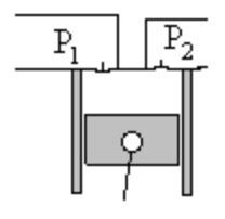
By the end of compression, the chamber is in communication with the discharge circuit so that the compressed gas at pressure P2 can emerge. A new mass of gas at pressure P1 is then sucked into the inlet pipe, and so on, the operation of the machine is cyclical.
The organs that control the discharge or admission are, in piston compressors, valves operated automatically by pressure differences between the chamber and the discharge or admission manifold.
One denotes displacement Vs the volume swept by the piston between its two extreme positions, and dead space e Vs the minimum volume of the compression chamber. In the current achievements, e is the order of 3 - 5%.
Because of the existence of the dead space, displacement compressors have a particular characteristic: their apparent displacement is less than their geometric displacement. A certain mass of fluid remains trapped in the compressor at the end of discharge, which reduces the useful volume of the machine. We characterize the reduction of displacement by a quantity called the volumetric efficiency.
Low volumetric efficiency does not inherently pose a disadvantage in terms of energy; it merely indicates that the mass flow passing through the compressor is less than the theoretically corresponding displacement. However, it proves economically disadvantageous, as it necessitates oversizing of the cylinder for a given specification, thereby resulting in higher investment costs.
Types of problems and difficulties associated
The study of the compressors in a power system has very different levels of difficulty depending on the objectives that we pursue.
The most basic approach is to calculate the outlet temperature when the compression ratio and isentropic efficiency are known. If the flow-rate involved is also known, the compression work can be deduced directly.
The inverse problem is solved also simply: knowing the compressor inlet and outlet states, itis to determine the isentropic efficiency of the device.
To go further and determine the isentropic efficiency and the flow through a given displacement machine, we have to perform more complicated calculations, requiring a thorough knowledge of compressor operation.
We will call technological design calculations for determining the displacement of a compressor knowing the laws giving its volumetric and isentropic efficiencies.
This is by the way a general problem in energy systems studies: as long as one is satisfied to carry out cycle studies without trying to size the geometry of the components, the calculations are much simpler than when one wishes to closely analyze their internal behavior.
Once the displacement determined, allowing to geometrically characterize the compressor, another problem remains to be treated: that of its behavior when operating conditions differ from those used in the design.
We call this problem the study of its off-design behavior.
It can be a higher level of complexity than the technological design, because it may require solving large systems of nonlinear equations when several components are coupled together.
Elements of the theory of compression
Machines doing the compression or expansion of a fluid have a very compact design for reasons of weight, size and cost. For similar reasons, they rotate very fast (several thousand revolutions per minute). Each parcel of fluid remains there very shortly.
Moreover, the heat exchange coefficients of gases have low values. Short residence time, small areas of fluid-wall contact, and low exchange coefficients imply that the heat exchange is minimal and that the operation of these machines is nearly adiabatic.
Under these conditions, the ideal reference process is the reversible adiabatic, i.e. the isentropic process.However, in a real machine, irreversibilities take place, mainly due to viscous friction and shock. They have the effect of increasing the fluid temperature and entropy. In an entropy chart, the evolution deviates from the theoretical isentropic vertical (see figure below).
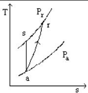
Real adiabatic compression
To calculate the work put into play in a real adiabatic compression, there are two ways to operate:
The first is to introduce an efficiency eta s called isentropic or adiabatic efficiency, which is determined experimentally, as the ratio of isentropic work to real work;
The second way is to introduce the concept of polytropic.We refer the interested reader to the thematic page on compressors .
Losses in displacement compressors
In a displacement compressor, two types of losses are generally considered:
Those which reduce the compressor capacity, which are represented as we have said by the volumetric efficiency;
Those from thermodynamic and mechanical irreversibilities taking place in it, which are often characterized by the isentropic efficiency.
In the current state of our knowledge, the determination of these two types of losses can only be carried out globally and experimentally.
Volumetric efficiency lambda
Analysis and experimentation have shown that lambda can be written as follows, the two biggest losses being in first place beta3, then beta1:
beta1 is the loss due to dead space.
beta2 the loss due to pressure drop in the intake and discharge manifolds;
beta3 the losses due to wall effects (thermal shunt);
beta4 the losses by leakage (at the piston rings and valves);
beta5 the loss due to pressure drop in the inlet and outlet valve.
There is a limit compression ratio beyond which the compressor no longer provides any fluid flow. Physically, this means that at the end of expansion, mass contained in the dead space at pressure Pasp occupies the entire volume of the cylinder, so that the compressor can no longer suck the upstream gas.
The set of all losses combine to give volumetric efficiency laws of variation with respect to compression ratio and to rotation speed which look like in figures below.
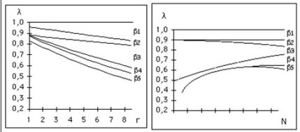
At constant compression ratio, they show an optimum at fairly high speed. Indeed, at low speeds, wall effects (beta3) and leakage (beta4) are relatively large, and drop when speed increases. However, at high speed, pressure drop in collectors (beta2) and especially valves (beta5) plays an increasing role.
Isentropic efficiency eta
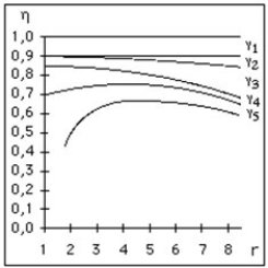
Three sources of losses linked to the previous ones mainly affect compression efficiency, which can be written:
wall effects (gamma3) are very disadvantageous because they greatly increase the compression work by deforming the isentropic;
losses due to valves (gamma5) come next, followed by default leakage losses (gamma4).
At a given speed, the shape of the compression efficiency law as a function of the compression ratio is given in figure 3.1.3. It shows the existence of a maximum at compression ratios rather low (3 to 5).
At a given compression ratio, when speed varies, compression efficiency goes by a maximum close to that of volumetric efficiency.
All of these phenomena are extremely complex to model, so we usually just adjust numerical models to represent the behavior of displacement compressors.
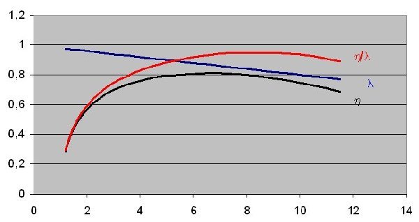
Generally, the volumetric efficiency has a substantially linear decrease as a function of thecompression ratio.
The figure below shows the shape of the isentropic efficiency and volumetric efficiency for a piston compressor.
Practical method of calculation and representation in Thermoptim
Determining the compressor outlet state
If we choose the isentropic efficiency approach, well suited for a displacement compressor, the sequence of steps for calculating a compression with the first approach can be stated as follows:
1) we must first calculate the entropy at suction s(Pa, Ta);
2) we must then reverse in Ts the entropy equation s(Pr, Ts) = s(Pa, Ta);
3) we must calculate the work corresponding to the isentropic process Dhs = h(Pr, Ts) - h(Pa, Ta);
4) we deduce the outlet enthalpy hr = h(Pa, Ta) + Dhs/eta , eta being the isentropic efficiency;
5) Finally, we obtain the discharge temperature Tr by reversing the equation h(Pr, Tr) = hr
Representation inThermoptim
The icon of a compressor in Thermoptim is:
The (phenomenological) compressor screen offers several thermodynamic settings:
if the compression is adiabatic, we can choose an isentropic or polytropic reference. We must then enter the value of the isentropic or polytropic efficiency
if the compression is not adiabatic, the calculation is then imperatively polytropic. You must enter the values of the polytropic efficiency and exponent

Thermoptim compression screen
As noted above, we can generally assume that the compression is adiabatic.
Using this screen requires that you provide on the one hand the value of the isentropic efficiency (in our case) or polytropic, and also that of the flow, either directly or through the upstream component if one exists.
When trying to accurately represent the behavior of a given compressor, it is necessary to characterize it by:
Its displacement;
The law of volumetric efficiency;
The law of isentropic efficiency.
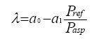
Volumetric efficiency law
Given the pace of losses presented above, a first order polynomial law is enough to represent the evolution of the volumetric efficiency as a function of the compression ratio:
Isentropic efficiency law
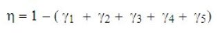
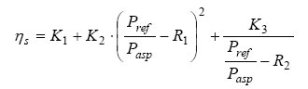
To properly represent the isentropic efficiency h, we need more parameters. The law we will retain uses 5:
To size a compressor, it is necessary to know these laws. Identification of their parameters can usually be made on the basis of data provided by the manufacturer.
Progressive and comprehensive study of a compressor
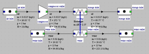
To illustrate what has just been presented, we will study the behavior of a piston air compressor that fills a compressed air storage of given volume at variable pressure. The compressed air is cooled before storage with a water exchanger of the type which is shown in the breadcrumb trail on heat exchangers .
The compressor sucks an air flow of 0.66 kg/min (11.738 g/s) at a bar and 26.85 °C, and compresses it at 5 bar.
Determination of the isentropic efficiency knowing the outlet state
We would like to know the value of the isentropic efficiency leading to an outlet temperature of 275 ° C.
The system can be easily modeled in Thermoptim and leads to a diagram of the type of the figure below, which differs from that studied in the breadcrumb trail of heat exchangers by the addition of the compressor.
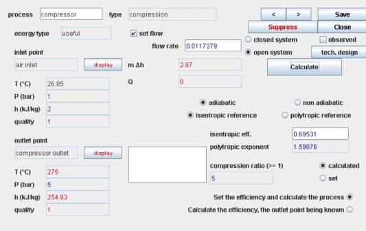
To determine the isentropic efficiency leading to the outlet temperature is chosen, we must select option "Calculate the efficiency, the downstream point being known" after having set the "outlet compressor" point, as shown in figure below.
The value obtained is eta = 0.69531.
Calculation of displacement volume for a compressor
To size the compressor, we must have the parameters of the equations giving the volumetric and isentropic efficiencies.
We assume here that they have been determined from data provided by the manufacturer.
The calculation of the compressor corresponds to the steps below:
the volumetric and isentropic efficiencies lambda and eta are calculated from their equations
If you know the rotation speed, the displacement and the volumetric efficiency, the flow rate can be calculated: Vvol = lambda N Vs / 60
Knowing the density at the inlet v, we deduce the mass flow: m = Vvol / v = lambda N Vs / 60 /v
In design mode, we determine the rotation speed to provide the desired flow or the displacement corresponding to a given rotation speed. The calculation is performed taking into account the inlet and outlet pressures and the flow value entered in the flow-rate field of the compressor.
In off-design mode, the compression ratio determines lambda and eta, which gives the compressor flow rate and outlet temperature.
Using the generic driver
When you simply want to make the technological design of a project that implements components of the Thermoptim core, it is possible to automatically create technological screens using the generic driver, which avoids having to program one.
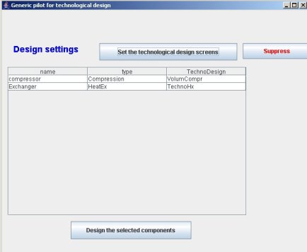
Open the Thermoptim project, and load the generic driver by choosing from among the list of drivers, the one whose title is "generic techno design driver", then click "Set the technological design screens".
Warning: the generic driver requests that the diagram and the project are both loaded into Thermoptim.
Two lines appear corresponding to the exchanger and the compressor, as in the figure below. Select that of the compressor.
Its type is by default Compression, and its TechnoDesign VolumCompr. Since it is a displacement compressor, they are perfect. Double-clicking on this line would change the type of TechnoDesign, but this is not necessary.
To display the technological design screen, the simplest here is to open the compressor process and click on "tech. design" located just above the "Calculate" button.
Technological design screen
The compressor technological design screen is given in figure below.
The blue fields on the left side of the compressor technological screen allow you to enter the compressor characteristics:
the two volumetric efficiency parameters a0 and alpha;
the five isentropic efficiency parameters K1, K2, K3, R1 and R2;
the reference speed (for which the five parameters were determined);
the swept volume at full load Vs (m3).
Enter in these fields the parameter values, select "Calculate Vs" so that Thermoptim know that this value must be calculated, then return to the generic driver screen, and click "Design the selected components".
The fields on the right side of the screen show calculated values of isentropic efficiency, mass flow and volumetric efficiency.
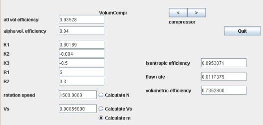
Compressor technological screen
The displacement (0.0055 m3) was determined on the basis of the flow entered the compressor process, and other values from the parameter values. Once the displacement recalculated, the "Calculate m" option is selected because it corresponds to the normal calculation mode of this TechnoDesign.
The files for this example are available for download .
We did not discuss here the design of the heat exchanger, which is explained in detail in the exchangers breadcrumb trail.
Off-design calculations
In off-design mode, we generally know the rotation speed and displacement. The compression ratio and inlet specific volume allow us to calculate the new values of volumetric and isentropic efficiencies, and to deduce the outlet temperature, flow ratey and the corresponding compression work.
To illustrate this type of calculation, we will now study the behavior of the air compressor, when used to fill a compressed air storage of given volume at variable pressure.
We are going to make it in three steps:
make a driver that will automate the recalculation of the compressor equipped with a cooling exchanger to simulate its behavior for different values of discharge pressure;
numerically identify the parameters of laws allowing us to express the changes in the compressor outlet temperature, flow rate and compression work of depending on the discharge pressure;
build a spreadsheet that will provide the evolution of the state of the compressed air storage over time.
Role of the driver
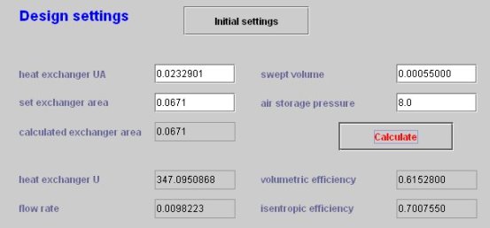
To achieve the desired results, we must build a driver, whose screen may look like below. It allows us to vary the compression ratio to get the major value changes when the tank pressure varies by operating as follows:
Update the outlet compressor pressure
Calculate the compressor volumetric efficiency
Calculate the compressor isentropic efficiency
Recalculate the compressor and downstream process
Update the heat exchanger inlet and outlet points
Determinate U and AU update and recalculate the heat exchanger in off-design mode (in various iterations since U depends on the average temperatures of the fluids, and therefore those of outlet points)
Update the simulator and displays
The results shown below correspond to a compression ratio equal to 8. The rate fell slightly, due to the law of volumetric efficiency, and isentropic efficiency increased slightly.
Note that in this example the behavior of the compressor is independant, once the compression ratio set, of that of the downstream heat exchanger: there is no system coupling, at least for a given operating point .
The design of the driver is facilitated: there is no nonlinear coupling equation system to solve.
We will not detail here the driver program, which is explained in Volume 4 of the reference manual, which we advise the interested reader to refer to.
Exploitation of simulation results
Once the driver made it very easy to vary the compression ratio for determine the main variables when the tank pressure varies.
They can be used with the Excel macro post-processing Thermoptim simulation files presented in Volume 1 of the reference manual. Simply save the project file under a different name after each simulation, then load these files into the macro and extract the values of interest.
The figure below shows, depending on the storage pressure, changes in the compressor isentropic efficiency, compression work, intake air flow, temperature of air entering the tank, the exchanger load and UA.
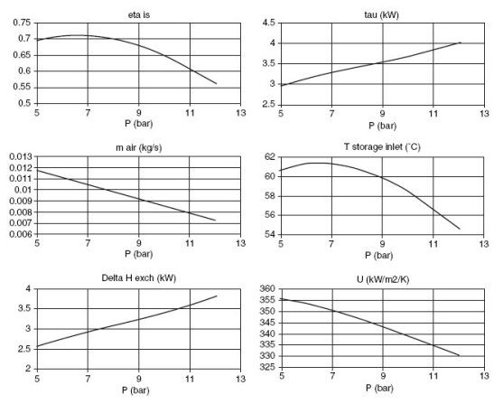
Influence of discharge pressure on the compressor performance
Between 5 and 12 bar, h and U vary by 22% and 7%. As the curves are in some cases far from linear, overly simplistic approaches are not enough, which demonstrates the interest of our approach.
Using the model to simulate the filling of a compressed air storage
The results of the above figure can be used to simulate the filling of a compressed air storage. Thermoptim only providing results for steady state operation, the simplest is to develop a second model, solved with Excel.
Its equations are:
the mass of air contained in storage M is equal to the initial mass plus the integral of flow;
The internal energy U is equal to the initial internal energy plus the integral of the product of the flow by the air enthalpy leaving the cooler, less the integral of the loss by convection with ambient air;
The storage temperature is inferred from its internal energy;
The pressure is determined by the ideal gas law.
For the flow rate, the compression work and the temperature of the air entering storage, we have just to make polynomial regressions from simulations previously done with Thermoptim. Depending on the compression ratio r, the equations are obtained:
m = -0.006 r + 0.0149
Tair = 0.01 r3 - 0.4735 r2 + 4.9142 r + 46.699
tau = 0.0019 r3 - 0.0484 r2 + 0.5322 r + 1.2806
The look of the results is given figure below, for a storage of a half m3 (diameter 80 cm, length 1 m), powered by a compressor of displacement Vs = 0.55 l. The pressure and temperature in storage, its mass and the of compressor work are shown versus time in seconds.
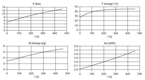
Filling of the compressed air storage
The files for this example are available for download
CRC_we_14, CRC_we_15
