Dynamic compressors
Example of axial dynamic compressor
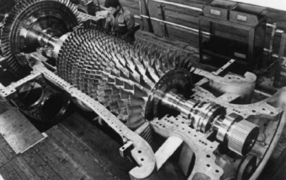
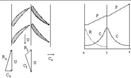
Velocity profile
In a dynamic compressor, the evolution of the fluid is increased pressure, which, for a subsonic regime, requires that the section of the vein is increasing, while the velocity decreases. Evolution is a two time process (Figurebelow): in the impeller, the relative velocity drops sharply, while the absolute velocity increases. The stator (diffuser) then slows the absolute velocity down.
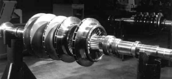
Simililarity
To study the operation of the dynamic compressor, we use the concept of similarity, which allows one to identify adequate dimensionless quantities. The figure below shows the assembly in series of five similar centrifugal compressors.
Modeling assumptions
Machines doing the compression or expansion of a fluid have a very compact design for reasons of weight, size and cost. For similar reasons, they rotate very fast (several thousand revolutions per minute). Each parcel of fluid remains there very shortly.
Moreover, the heat exchange coefficients of gases have low values. Short residence time, small areas of fluid-wall contact, and low exchange coefficients imply that the heat exchange is minimal and that the operation of these machines is nearly adiabatic.
The reference process for compression or expansion with work is the perfect or reversible adiabatic, i.e. the isentropic.
However, in a real machine, irreversibilities take place, mainly due to viscous friction and shock. They have the effect of increasing the fluid temperature and entropy. In an entropy chart, the evolution deviates from the theoretical isentropic vertical (see figure below).
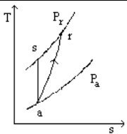
Real adiabatic compression
Calculation method
To calculate the work put into play in a real adiabatic compression, there are two ways to operate:
The first is to introduce an efficiency eta s called isentropic or adiabatic efficiency, which is determined experimentally, as the ratio of isentropic work to real work;
The second way is to introduce the concept of polytropic. For this, we assume that the irreversibilities are uniformly distributed over the entire process. We can then derive a differential equation, assuming that the isentropic efficiency keeps a constant value during any infinitesimal compression. By definition the polytropic efficiency is equal to this infinitesimal isentropic efficiency. This differential equation leads to a simple equation for a perfect gas:
The sequence of steps for calculating a compression with the first approach can be stated as follows:
1) we must first calculate the entropy at suction s(Pa, Ta);
2) we must then reverse in Ts the entropy equation s(Pr, Ts) = s(Pa, Ta);
3) we must calculate the work corresponding to the isentropic process Dhs = h(Pr, Ts) - h(Pa, Ta);
4) we deduce the outlet enthalpy hr = h(Pa, Ta) + Dhs/eta , eta being the isentropic efficiency;
5) Finally, we obtain the discharge temperature Tr by reversing the equation h(Pr, Tr) = hr
The icon of a compressor in Thermoptim is:
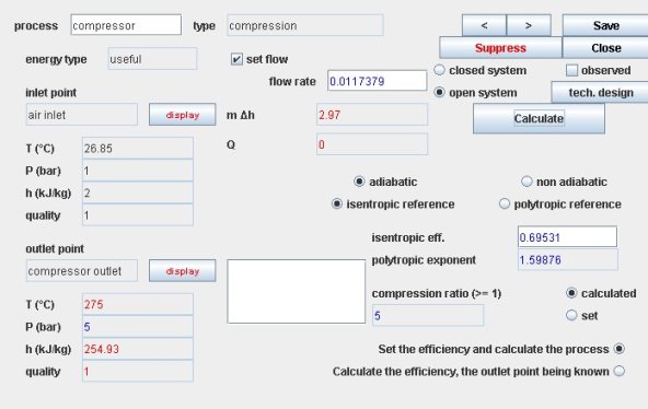
Thermoptim compression screen
The compressor screen offers several thermodynamic settings:
if the compression is adiabatic, we can choose an isentropic or polytropic reference. We must then enter the value of the isentropic or polytropic efficiency
if the compression is not adiabatic, the calculation is then imperatively polytropic. You must enter the values of the polytropic efficiency and exponent
Dynamic compressor performance map
For dynamic compressors the corrected mass flow is used as abscissa. The ordinate is the pressure ratio or the isentropic efficiency. The corrected rotation speed is still used as parameter.
The corrected rotation speed strongly influences the performance of dynamic compressors. This is easily explained considering that in such a machine, energy is transmitted to the fluid by the rotor in the form of kinetic energy. At most, this energy is 1/2 U2, that is to say, is proportional to N2. It is therefore natural that the sensitivity of these machines to regime change is dramatic.
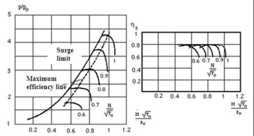
In addition, fluid mechanics tells us that the fluid flow in the blades is destabilized here by the pressure gradient. As soon as one deviates too much from the nominal operating conditions, there is a significant risk of stream separation along the blades. Besides a strong sensitivity of isentropic efficiency, this results in a double limitation of range of use of the machine: the risk of surge at low flow (which depends on the network in which the compressor discharges), and stalling on the side of higher flow rates. Some flexibility is indeed possible in this type of machine only if you can freely adjust the rotation speed and possibly the angle of incidence of certain rows of blades (guide vanes).
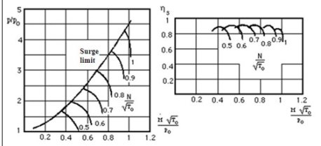
Axial compressor performance map
Characteristics of axial compressors are less steep than those of centrifugal compressors, making them less stable. The compression ratios per stage that can provide axial compressors are relatively low, generally between 1.2 and 2.
Book references
Thermodynamcs ofcompression
An excerpt of the textbook chapter is freely downloadable with the agreement of CRC Press
Available Diapason session
n° | content | steps | soundtrack duration |
|---|---|---|---|
S11En | 16 | 5 mn 45 s |
