Turbines
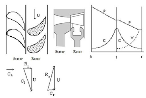
Velocity profile
In a turbine, the evolution of the fluid is an expansion. The compressible flow equations indicate that for a subsonic regime, the section of the vein should decrease, and the velocity increase. This evolution takes place in two steps (Figure below): in the stator, the absolute velocity increases, while in the impeller the relative velocity increases, and the absolute velocity decreases.
To study the operation of the turbines, we use the concept of similarity, which allows one to identify adequate dimensionless quantities.
Degree of reaction
We call the degree of reaction the fraction of the enthalpy change that takes place in the rotor
In a turbine stage, pure reaction is impossible. Two limiting cases frequently arise:
impulse turbines, in which the degree of reaction is equal to 0: any expansion of the fluid is then carried out in fixed blades or nozzles, at the inlet of the wheel, and the inlet and outlet pressures of the rotor are equal;
reaction turbines, where the degree of reaction is equal to 0.5: the expansion is then evenly distributed between the nozzle and the wheel.
Each of these two types of turbine has advantages and disadvantages of its own.
The impulse turbines are generally used for head stages of multistage sections or for small capacity units, while reaction turbines are proving well suited for the low-pressure sections.
Indeed, a first advantage of using impulse turbines in the high pressure sections is that the entire expansion being made in the stator, the rotor is not subjected to a high pressure difference, which limits the mechanical constraints. A second advantage is that the flow in these turbines can be reduced by using partial injection, which is to only supply a fraction of fluid in the stator vanes. This type of operation is made possible in this case because the pressure is the same on both sides of the rotor, and no parasitic flow is expected in the non-injected parts.
However, the efficiencies of these turbines are slightly (2-3%) worse than those of reaction turbines, which are subjected to significant axial thrust, and do not use partial injection.
Because irreversibilities taking place in the top stages are partially recovered in subsequent stages, we can tolerate that their efficiency is slightly lower, which allows us to use impulse turbines in this case.
Different types of steam turbines
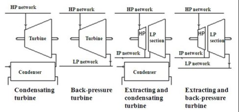
Depending on their use, there are four broad categories of turbines:
condensing turbines, where steam is completely expanded at a pressure of about 0.02 to 0.04 bar, and then liquefied in a condenser cooled by ambient air or by water. This type of turbine is mainly used in the power production facilities;
lback-pressure turbines, in which vapor pressure is expanded from HP pressure (> 40 bar) at low pressure (about 4 bar). This type of turbine allows production of mechanical power or electricity thanks to the high temperature and pressure that can be obtained in a boiler, while using the residual enthalpy for various processes;
extracting and condensing turbines, in which vapor undergoes partial expansion at an intermediate pressure (about 20 bar) in a high pressure section. One part is directed to a user network, while the rest of the steam is expanded in a low-pressure section, as in a condensing turbine. This type of turbine finds an important field of application in cogeneration plants whose requirements for heat are likely to vary considerably over time;
extracting and back-pressure turbines, in which steam escapes at low pressure in a LP network instead of being condensed.
Modeling assumptions
Machines doing the compression or expansion of a fluid have a very compact design for reasons of weight, size and cost. For similar reasons, they rotate very fast (several thousand revolutions per minute). Each parcel of fluid remains there very shortly.
Moreover, the heat exchange coefficients of gases have low values. Short residence time, small areas of fluid-wall contact, and low exchange coefficients imply that the heat exchange is minimal and that the operation of these machines is nearly adiabatic.
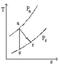
The reference process for compression or expansion with work is the perfect or reversible adiabatic, i.e. the isentropic.
However, in a real machine, irreversibilities take place, mainly due to viscous friction and shock. They have the effect of increasing the fluid temperature and entropy. In an entropy chart, the evolution deviates from the theoretical isentropic vertical (see figure below).
Real adiabatic expansion
Calculation method
To calculate the work put into play in a real adiabatic expansion, there are two ways to operate:
The first is to introduce an efficiency eta s called isentropic or adiabatic efficiency, which is determined experimentally, as the ratio of real work to isentropic work;
The second way is to introduce the concept of polytropic. For this, we assume that the irreversibilities are uniformly distributed over the entire process. We can then derive a differential equation, assuming that the isentropic efficiency keeps a constant value during any infinitesimal compression. By definition the polytropic efficiency is equal to this infinitesimal isentropic efficiency. This differential equation leads to a simple equation for a perfect gas:
The sequence of steps for calculating an expansion with the first approach can be stated as follows:
1) we must first calculate the entropy at suction s(Pa, Ta);
2) we must then reverse in Ts the entropy equation s(Pr, Ts) = s(Pa, Ta);
3) we must calculate the work corresponding to the isentropic process Dhs = h(Pr, Ts) - h(Pa, Ta);
4) we deduce the outlet enthalpy hr = h(Pa, Ta) + Dhs*eta , eta being the isentropic efficiency;
5) Finally, we obtain the discharge temperature Tr by reversing the equation h(Pr, Tr) = hr
The icon of a turbine in Thermoptim is:
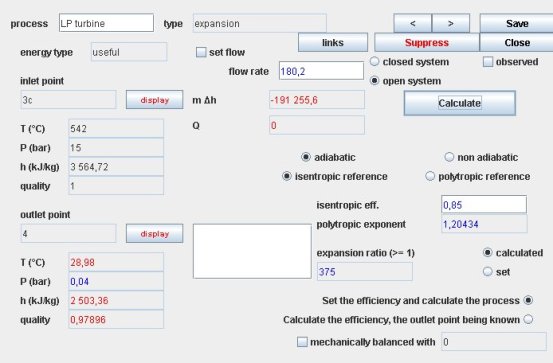
Thermoptim expansion screen
The turbine screen offers several thermodynamic settings:
if the expansion is adiabatic, we can choose an isentropic or polytropic reference. We must then enter the value of the isentropic or polytropic efficiency
if the expansion is not adiabatic, the calculation is then imperatively polytropic. You must enter the values of the polytropic efficiency and exponent
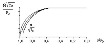
Performance map of a turbine
In the case of a turbine it is conventionally the pressure ratio which is used as abscissa. As ordinate, we find the corrected mass flow or isentropic efficiency of the machine. The curve parameter is still the corrected rotation speed, which plays a secondary role.
We can see the flexibility of turbines to adapt to various operating conditions: efficiency tends to deteriorate only when we dramatically reduce the pressure ratio or the speed. This flexibility is particularly due to the flow stability in the blades due to the gradient of pressure therein. But what is most remarkable is the stability of the flow for the high pressure ratios, which comes from the supersonic regime, which takes place in at least part of the machine (the flow is choked at the place where the speed of sound is reached).
The limiting value reached by the flow, when the pressure ratio exceeds the critical report, is called critical flow. It is proportional to the throat section, which is obviously independent of the rotation speed, which explains the weak influence of this parameter.
Book reference
An excerpt of the textbook chapter is freely downloadable with the agreement of CRC Press
Available Diapason session
n° | content | steps | soundtrack duration |
|---|---|---|---|
S11En | 16 | 5 mn 45 s |
