This second section introduces thermodynamic concepts whose knowledge is essential to to model energy systems.

After having started by a discussion on the performance of compressors and turbines used in a gas turbine, we will present the concepts of thermodynamic system and state.

The energy exchanges between a thermodynamic system and its surroundings will then be studied, which will make it possible to state the First Law of thermodynamics in a closed and then open system.

We will show that the four main elementary functions identified in the previous section correspond to three reference processes undergone by the fluids which pass through the machines, each declining a particular case of application of the First Law of thermodynamics that we will present.

In a compressor, the ratio of the discharge pressure to the suction pressure is called the compression ratio, and, in a turbine, its inverse is the expansion ratio.

Study of compression

When you compress a gas, it heats up, as everyone can see when inflating a bicycle tire. The compression of a gas is therefore accompanied by a simultaneous increase in its temperature and pressure. This unavoidable heating of the gas unfortunately results in additional compression work, more or less important depending on the quality of the compressor.

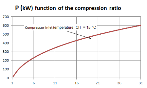
To fix ideas, let us take a look at the work required by the compressor of a gas turbine. the figure above shows, for a gas turbine of common characteristics crossed by a flow rate of 1 kg/s, the variation of the compression power as a function of the compression ratio, for a compressor inlet temperature CIT of 15 °C.

For example, for a compression ratio of 6, the power required is almost 220 kW, and for a compression ratio of 21, it is worth 500 kW.

As can be seen, the higher the compression ratio, the more work required for the compressor.

The performance of a gas turbine compressor is very sensitive to the value of the suction temperature of the fluid, here the outside temperature. The latter evolving between winter and summer from - 5 °C to about 35 °C, the compression power input varies by more or less 7% around its average value, for a compression ratio of 16, the minimum power to be supplied corresponding to winter, as shown in the figure below.

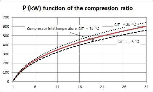
The performance of a gas turbine compressor is very sensitive to the value of the suction temperature of the fluid, here the outside temperature. The latter evolving between winter and summer from - 5 °C to about 35 °C, the compression power input varies by more or less 7% around its average value, for a compression ratio of 16, the minimum power to be supplied corresponding to winter, as shown in Figure 2.22.

The influence of the suction temperature on the compression power explains why it is always preferable to compress a gas at the lowest possible temperature, which leads to cooling it if it is technically possible.

It can be shown that the compression work of an ideal gas is on the one hand proportional to the temperature of the suction fluid (expressed in Kelvin), and on the other hand an increasing function of the compression ratio. If Ps and Pd designate the suction and discharge pressures of the compressor, and if CIT is the compressor inlet temperature, in °C:

tau= (TIC + 273.15) fc(Pd/Ps).

When the fluid cannot be assimilated to an ideal gas, this relationship remains valid as a first approximation.

Study of expansion

The work produced by a compressed gas being expanded in a turbine is all the more important as its temperature is high: it is given as a first approximation by a relation similar to that of a compression, if TIT is the turbine inlet temperature, in °C:

 = (TIT + 273.15) fd(Pd/Ps).

Let us illustrate this point by studying the expansion that takes place in the turbine of a gas turbine. The higher the turbine inlet temperature TIT (equal to the temperature at the outlet of the combustion chamber), the higher the power output. The influence of this value is significant: for an expansion rate of 16, a variation of 100 °C in the temperature reached at the outlet of the combustion chamber causes the power output of the turbine to vary by more or less 8% around its average value (Figure below).

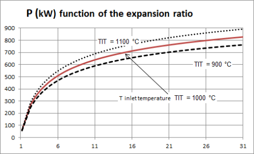
For example, for an expansion ratio of 6, the power output is 500 kW, and for a compression ratio of 16, it is worth about 720 kW.

Study of the whole gas turbine

Now let us take a look at what is going on in the whole machine, the assembly of a compressor, a combustion chamber and a turbine.

In the combustion chamber, the chemical energy supplied to the cycle in the form of fuel is converted into thermal energy which is used to bring the hot gases to the high temperature TIT.

Since the combustion chamber is roughly isobaric, the pressures upstream and downstream are the same. Since atmospheric pressure prevails at the compressor intake and the turbine exhaust, the compression and expansion ratios are equal. We will therefore only consider in the following the first of these parameters.

The figure below shows, for a gas turbine of common characteristics (compressor inlet temperature CIT of 15 °C and turbine inlet temperature TIT of 1000 °C), crossed by a flow rate of 1 kg/s, the compression power (solid line), the power delivered by the turbine (dashed line), and net power produced by the machine (dotted line), as a function of the compression ratio.

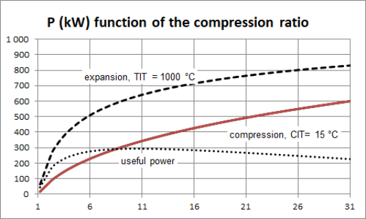
For example, for a compression ratio of 6, the compression power is around 220 kW, and the useful power output is 270 kW.

If the compressed air was expanded at the temperature reached at the end of compression, without additional heat, the balance would be negative because of the losses which take place in the compressor and the turbine.

It is only because the constant pressure combustion reaction brings the gases to high temperature, that the work provided by the turbine is greater than that which is absorbed by the compressor.

The maximum net power is obtained here for a compression ratio of around 10, but the optimum is fairly flat.

The influence of the inlet temperatures of the compressor and the turbine is even more noticeable on the overall performance of the machine than on the components alone, because the useful power is equal to the difference between the power required by the compressor and that deliverd by the turbine. For example, the useful power drops by 31.5% when the outside temperature rises from - 20 °C to + 20 °C.

Conclusions

This study allowed us to highlight the influence of the main characteristics of the machine (compression ratio, inlet temperatures in the compressor and in the turbine) on the performance of a gas turbine.

It has shown that it is preferable to cool a gas as much as possible before compressing it, and to heat it as much as possible before expanding it, the energies put in play being proportional to the absolute temperature at the inlet of each component.

It also showed the influence of the compression or expansion ratio on the performance of the machine.

These are points to which we will return later.

Note that a common mistake is to assume that the pressure should increase in the combustion chamber, as in those which constitute closed systems.

Indeed, the phenomenon is similar to that which takes place in a wall-mounted gas boiler, the combustion of which takes place at atmospheric pressure, the system being open, or else in the devices that everyone knows, used for cooking or heating, whether it be gas stoves, fireplaces or others. They have no element varying the pressure, which therefore remains constant.

To be able to model the energy systems which interest us, it is necessary to introduce a certain number of notions of thermodynamics.

Our aim being to adopt as simplified an approach as possible, we will limit theoretical developments as much as we can.

Study these concepts well, even if they seem a little vague at first. Their meaning will become increasingly clear to you as you have the opportunity to put them into practice.

Notions of thermodynamic system and state

Let us begin by introducing the concept of thermodynamic system, which represents a quantity of matter isolated from what we call the surroundings by a real or fictitious boundary. This system concept is very general in physics and is found especially in

mechanics.

These three concepts are fundamental and will be widely used later.

By way of illustration, the figure below shows that it is possible to define the boundary of the "steam power plant" system in several ways, represented by a rectangle drawn in thin lines.

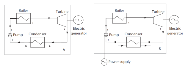
The usual definition, identified by the letter A, is illustrated by the left part of the figure. The flows crossing the boundary are the hot gases coming from the hot source and the cooling fluid coming from the cold source. The mechanical power leaving the system is that which drives the electric generator. It implicitly assumes that the compression work of the pump is taken from that provided by the turbine.

The second definition of the system, identified by the letter B, is illustrated by the right part of the figure. It assumes that the compression work of the pump is not taken from the work provided by the turbine, but brought in the form of electricity by the surroundings. We will see below the implications of this change of boundary on the calculation of the energy balance of the system.

Remember that you must always specify the boundary of the system in question.

State variables and functions

A second very important notion in practice is that of state. It allows you to characterize a system concisely.

The notion of state of a system represents "the minimum information necessary to determine its future behavior".

This state is characterized by what is called a set of state variables making it possible to completely characterize a system at a given time.

In mechanics, position variables and speed are state variables.

For a simple thermodynamic system like a particle of matter in a pure fluid, there are several sets of state variables that meet this definition. The most used in the literature are the following pairs: (pressure, temperature), (pressure, volume), (temperature, volume).

For more complex systems, it may be necessary to add two other broad categories to these state variables:

• chemical variables;

• electrical variables.

A state function is a quantity whose value depends only on the state of the system, and not on its history.

We will note with a d an infinitesimal evolution of a state function: for example dP for a small pressure variation

However, during the evolution of a thermodynamic system, many quantities depend not only on the initial and final states of the system, but also on the way in which evolution takes place.

These quantities are often called path functions, to indicate this dependence . This is the case of the work brought into play or the heat exchanged at the boundaries of the system. We will note with  an infinitesimal evolution of a path function: for example W for a small variation of work

In the general case, the calculation of these path functions is more complex than that of the state functions.

Open and closed systems

In thermodynamics, we are often led to distinguish two types of systems: closed systems, which do not exchange matter with the surroundings, and open systems which exchange matter (Figure below).

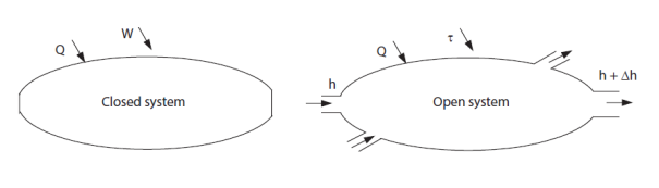
This distinction is important because thermodynamic properties are not expressed in the same way in closed systems and in open systems. Paradoxically even, they are generally easier to calculate for open systems, although they involve a transfer of matter.

At this stage of our presentation, it is important to note that the open or closed character of a system depends on the boundaries that we choose to define it, which can induce small semantic difficulties.

Self assesment activities

These self-assessment activities will allow you to test your understanding of these concepts:

• State and path functions, cat

• Differences between closed system and open system, gfe

We will now study the energies that components of the energy systems exchange with their surroundings, and state the First Law of thermodynamics, fundamental in practice.

In what follows, unless otherwise indicated, we will reason in a closed system on a quantity of material of 1 kg, and, in an open system on a working fluid flow of 1 kg/s. This will allow us to lighten the notations by not showing the quantities or flow rates involved.

It is essential to note that thermodynamic systems associated to the components we are interested in, only exchange energy with the surroundings in two distinct forms:

• heat by heat exchange on the system boundaries. It is usually denoted by Q;

• work, by action of pressure forces on the boundaries, the work of gravity forces being neglected. This work is usually denoted W in closed and tau in open systems where it is often named shaft work.

We indicated previously that, to calculate these two forms of energy brought into play in a process, it is not enough to know the initial and final states of the system. It is also necessary to know the path followed during the process.

This is a classic problem: how can we calculate the global change of a variable during a process?

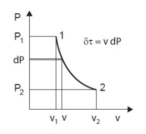
The solution, if it exists, concerns differential calculus. It consists in decomposing the process into what are called elementary processes, for which we can write the equations of physics by considering that the quantities remain constant. The variation in properties is then taken into account by "integrating" the differential equations thus written, which makes it possible to express the laws followed by the whole process. In the context of this simplified presentation, we limit ourselves to indicating how it can be done, but there is no need to go further (Figure below).

One can also easily show that in an open system, for an infinitely small change, and Q are given by the following equations:

= v dP, or dP = ρ δtau

The useful work received by the movable walls of the system is equal to the product of the mass volume of the fluid by the elementary variation of the pressure within it. Applied to a compressor stage, this expression indicates that the compression ratio achieved is equal to the product of the density ρ of the fluid by the work communicated to the machine shaft.

The second equation is:

δQ = Cp dT – v dP

The latter expression simply expresses an experimental fact, which is an essential basis of compressible fluid thermodynamics: heat δQ exchanged with the surroundings causes a linear change in the thermodynamic state of the system, here characterized by two state variables, temperature T and pressure P.

If the pressure remains roughly constant, which is the case in most heat exchangers, dP = 0 and the variation in temperature of the fluid is proportional to the heat supplied to the system.

In the context of this presentation, we will not seek to solve these equations: we will determine the energies put into play using well-chosen state functions.

Let us emphasize an important point: heat Q and temperature T should not be confused, even if relations exist between the two concepts:

- the temperature is a measure of the degree of agitation of the molecules of the working fluid: the more they are agitated, the higher its temperature;

- heat is a transfer of thermal energy from one system to another when there is a temperature difference between them.

When a pure fluid condenses, its temperature remains constant, while it exchanges heat with the surroundings.

Let us now come to the First Law of thermodynamics.

We define the internal energy U of a system as the sum of the microscopic kinetic energies (comparable to the thermal agitation of particles) and the potential energies of microscopic interactions (chemical bonds, nuclear interactions) of the particles constituting this system. The internal energy corresponds to the intrinsic energy of the system, defined on the microscopic scale, excluding the kinetic or potential energy of interaction of the system with its surroundings, on the macroscopic scale, that which acquires a body because of its mass and speed.

The internal energy is defined with an arbitrary constant u0, often chosen such that U = 0 for T = 25 °C and P = 1 atmosphere. Its unit in the International System (SI) is the Joule, but it is also frequently expressed in kWh, knowing that 1 Wh = 1 Watt for 1 h = 1 J/s x 3600 s = 3600 J.

The fundamental law that governs the behavior of thermodynamic systems is the conservation of energy, known as the First Law.

It postulates that the variation of internal energy ΔU of a non-isolated system, interacting with its surroundings and undergoing an evolution, depends only on the initial state and the final state, which means that u is a state function.

The First Law indicates that, if the internal energy U of the system varies, it means that there is an exchange of energy with the surroundings in the form of work and / or heat, and that the sum of W and Q is equal to the variation of internal energy of the system. It can thus be written for a closed system in the form:

ΔU = W + Q

What is remarkable is that u is a state function, while the two functions W and Q are only path functions.

Let us clarify a point important in practice: by convention, in this course, we will consider that the energy received by a system is counted positively (its internal energy increases), and that given away to the surroundings is counted negatively.

For a closed system, the First Law can be stated as follows: the energy contained in a system which is isolated, or evolving in a closed cycle, remains constant whatever processes it undergoes. The various forms that the energy of a system can take: mechanical energy, heat energy, potential energy, kinetic energy, are all equivalent under the First Law. Let us recall that, in our case, only heat and work are taken into account.

In this form, this law is very intuitive and readily accepted: it is a conservation law which states that energy (like mass) is neither lost nor created.

Consider for example the thermal balance in winter of a house heated at a constant temperature of 18 °C (Figure below). To simplify the problem, we neglect the renewal of air, and assume that it is heated by electricity, so that no fluid enters or leaves it.

The whole constitutes a closed system. The house has heat losses towards the surroundings through its walls, the environment being colder, as well as, towards the ground. It may have gains due to sunshine.

The First Law indicates that the heating power is equal to the thermal power due to these losses minus the gains due to the sun.

To be exact, one must take into account the effects due to the thermal inertia of the house, which means that at certain times energy is stored in its walls and at others it is destocked and contributes to heating, but this reasoning is quite correct on average: the temperature of the house remaining constant, its internal energy does not vary, and all the heating energy that enters the house is equal to that which comes out due to thermal losses.

For a system consisting of a phase of mass m, U = m u, u being the internal mass energy

The unit of u is Joule/kg, but it is also frequently expressed in kJ/kg.

The internal energy, however, has meaning only if the system is closed, and needs to be generalized when considering a system in which matter enters and/or out of which it flows.

The principle of reasoning consists in following the evolution of a closed control volume in a periodic machine, and in calculating the work of external forces which is exerted during a cycle on all of its walls, by distinguishing the sections of passage of fluids (A1 and A2 at time t0, becoming B1 and B2 at time t0 + Δt in the figure below), the fixed walls, which obviously do not produce or receive any work, and the movable walls, on which a certain work is exerted, which is called "useful work", that is to say seen by the user.

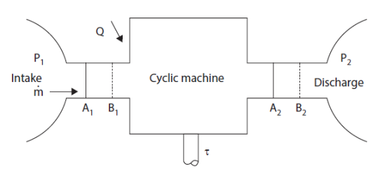
The work W exerted on a closed system can indeed be broken into two parts: one that is exerted on the mobile walls of the system if any, called shaft work tau, and one that is exerted on boundaries crossed by fluid coming out of the system and entering it. For open system components, which is the case for those that we are studying, this work, called flow work, equals - Δ(PV).

We therefore have: W = -Δ(PV)

Introducing a function called enthalpy H, such as ΔH = ΔU +Δ(PV), the First Law in open systems is written:

ΔH = + Q

The First Law is expressed as follows in open systems: the enthalpy change in an open system is equal to the sum of shaft work exerted on the moving walls and heat exchanged with the surroundings.

Enthalpy thus appears simply as a generalization in open systems of the internal energy in closed systems. In practical terms, just consider this state function as the energy associated with the system under consideration, neither more nor less.

As we will see later, this notion is fundamental in practice.

To illustrate the First Law in an open system, let us take two examples.

To begin with, consider a flat solar thermal collector. This figure shows the sectional view of such a collector. The absorber is composed of a metal plate on which are welded pipes in which the heat transfer fluid circulates. The heat losses towards the front of the collector are reduced by one or more glazings (2 in the figure below) and those towards the rear by an insulation.

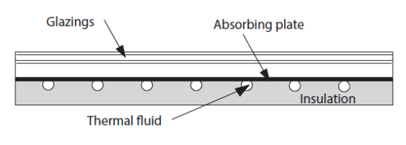
The incident solar flux is absorbed by the metal plate which is cooled on the one hand by the heat transfer fluid which heats up, and on the other hand by the thermal losses from the collector towards the surroundings.

The First Law indicates that the solar energy received by the collector is equal to the sum of the heat losses of the collector and the enthalpy variation of the heat transfer fluid.

Consider as a second example an electric hair dryer.

It consists of a fan placed upstream of an electrical resistance. When the hair dryer is running, the fan draws in air which is slightly compressed and passes through the electrical resistance which heats it. The jet of hot air is then used to dry the hair.

The First Law indicates that the electrical energy consumed by the device is equal to the change in enthalpy of the air passing through it.

For a system consisting of a phase of mass m, H = m h, h being mass enthalpy

The unit of h is Joule/kg, but it is also frequently expressed in kJ/kg.

The passage from specific energies to power outputs is done by simply multiplying the first ones by the mass flow rate of the fluid which crosses the system considered.

The unit of power is Watt, but it is also frequently expressed in kW

One Watt = 1 Joule/s

It is customary in physics to note a flow-rate by a point above the quantity considered.

Thus a mass flow is written , and an enthalpy power :

= h

As we said, for the sake of convenience and to simplify the notations, we will use, whenever possible, the unit of mass of the fluid considered.

Self-assessment activity

This self-assessment activity will allow you to test your understanding of the First Law:

First law in closed and open system, gfe

We will show in this section that the enthalpy variation of the fluid flowing through them is sufficient to determine the energy put into play in the four elementary processes that were identified previously.

The results presented here correspond to industrial reality: for various technological reasons, we do not know how to manufacture, in most cases, components capable of both transferring heat and achieving effective compression or expansion. We therefore separate the different functions to be performed.

Compression and expansion with work

As we have seen, expansion can be made with and without work production. In the first case, the machine most commonly used is the turbine. In the second case, it is a simple valve or a filter.

Machines doing the compression or expansion of a fluid have a very compact design for reasons of weight, size and cost. For similar reasons, they rotate very fast (several thousand revolutions per minute). Each parcel of fluid remains there very briefly.

Moreover, fluids brought into play in compressors and turbines are often gas whose heat exchange coefficients have low values.

Short residence time, small areas of fluid-wall contact, and low exchange coefficients imply that the heat exchange is minimal and therefore usually negligible; this is referred to as adiabatic.

It follows that the operation of these machines is nearly adiabatic: Q = 0.

In a compression or expansion adiabatic machine, writing the First Law in an open system shows that shaft work tau is thus equal to the change in enthalpy of the fluid Δh.

Expansion without work: valves, filters

There is a class of devices, such as the expansion valve of the refrigeration machine, where tau and Q are both zero, i.e. Δh = 0: they are static expanders such as valves and filters. The corresponding process is called an isenthalpic throttling or a flash expansion.

Heat exchange

Components which transfer heat from one fluid to another require large exchange areas, their heat fluxes being proportional to these areas. Technical and economic considerations lead to the adoption of purely static devices. For example, large bundles of tubes in parallel, traversed internally by one fluid while the other flows outside.

tau is zero because of the absence of movable walls.

In a heat exchanger, heat Q transferred or provided by one fluid to another is equal to its enthalpy change Δh.

Here we re-introduce the flow in the equation since there is one for each of the fluids and it is important not to confuse them.

Note also that, if we seek to increase the heat exchange between the two fluids, we also try to limit the heat transfer with the surroundings of the exchanger, which we will assume to be null.

If we note Δhh the variation in enthalpy of the hot fluid (which cools), and Δhc that of the cold fluid (which heats up), the First Law for the whole of the exchanger writes:

or

Combustion chambers, boilers

In a combustion chamber or boiler, there are no movable walls either, and tau = 0.

Heat Q transferred to the fluid passing through is equal to the enthalpy change Δh.

Regarding the working fluid, a boiler can thus also be considered as a heat exchanger.

The Diapason session S02En summarizes these topics.

The previous section showed that the determination of the enthalpy change of the fluid flowing through them is enough to calculate the energy put into play in these four elementary processes.

But this information is not sufficient to characterize them completely. The physical analysis of their behavior allows us to identify the reference processes corresponding to the operation of components that would be ideal.

It is then possible to characterize the actual process by introducing an imperfection factor, often called effectiveness or efficiency, which expresses its performance referred to that of the reference process. This way makes it much easier to understand the processes undergone by the fluid.

The choice of reference processes is based on analysis of physical phenomena that take place in the components: it is an absolutely essential modeling choice.

Lastly, as we shall see, the reference process is very useful when trying to plot the cycle studied on a thermodynamic chart.

Compression and expansion with work

We just saw that the compressors and turbines are machines in which heat exchanges with the surroundings are usually negligible, which is referred to as adiabatic.

Let us recall that the analyzes of these components have shown that, in such a process, the temperature and the pressure of the fluid vary simultaneously.

In a perfect compressor, that is to say one where the working fluid would not be subject to friction or shock, the heating of the fluid and the work required to obtain a given compression ratio would be minimal. In a perfect turbine, the cooling of the fluid and the work produced for a given expansion ratio would be maximum.

The reference process for compression or expansion with work is thus the perfect or reversible adiabatic. Its equation can be obtained by integrating the differential equation expressing that the heat exchanged is zero at any time, i.e. 0 = Cp dT – v dP. For a perfect gas, for which Pv = rT, the corresponding curve is easily obtained. It is given by law = Const with = Cp/Cv.

Expansion without work: valves, filters

For throttling or expansion without work conserving enthalpy (Δh = 0), the reference process is isenthalpic.

Heat exchange

Pressure drops correspond to the dissipation, by friction, of the mechanical energy of a moving fluid. They result in a drop in pressure and an internal heat supply.

Any pressure drop in heat exchangers must be compensated for by an additional compression work and / or results in a lower expansion work. As the penalty induced by pressure drops is expressed in the form of mechanical work, we always try to minimize it.

If the pressure drops are low, the pressure remains more or less constant and the heat exchanges can as a first approximation be assumed to be isobaric. The reference process is therefore the isobar.

Combustion chambers, boilers

Similarly, combustion chambers and boilers can usually be regarded as isobaric.

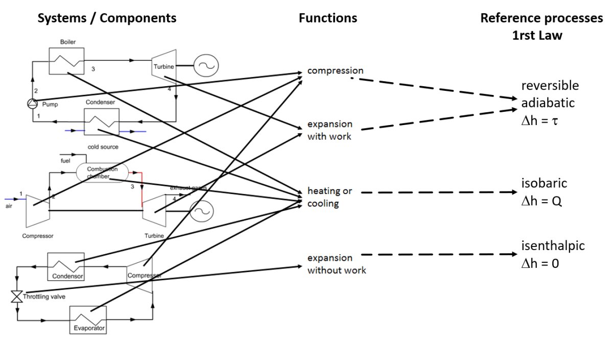
The figure below summarizes the links existing between the components of the systems studied, the functions and the reference processes. It illustrates the genericity of the reference processes which define the thermodynamic models corresponding to many technological components, and therefore their practical importance when one wishes to calculate the performances of the studied systems or to represent them in thermodynamic charts as we will see in the next section.

Self-assessment activity

This self-assessment activity will allow you to test your understanding of reference processes:

Reference processes, cat