Presentation of the Thermoptim optimization method
Note :
Optimization of complex energy systems by exergy methods
Limitations of conventional optimization approaches
Traditional approaches in thermodynamic systems optimization, valid for maximizing one by one the various components of a facility, remain insuffi cient to guide the designer in choosing the best configuration of the entire system.
Our system integration approach allows one to:
ensure greater consistency between all the energy needs and availabilities
reduce systemic irreversibilities induced by the assembly of system components and their relative positions.
The effectiveness of systems increases, thanks to improved internal regeneration
Work on this method for over ten years have resulted in:
several scientific publications
collaborations with industry (BABCOCK, EDF, Areva-Framatome)
a set of algorithms implemented in validated and Thermoptim
The power of the method depends to a large extent on the fact that it is not necessary to define the exchanger network beforehand. It is only built when the optimum has been found.
Implementation of the method
Once the system is modeled the method is carried out in four steps,
The first step consists of selecting the streams that are to be taken into account by the pinch analysis algorithms. The streams can be grouped into two categories: Hot streams, or availabilities, which must be cooled and that release heat, and cold streams, or needs, which must be heated. The streams are selected from the simulator, and the streams are generally exchange-type processes, or thermocouplers.
Once the streams have been selected, the second step, called "pinch minimization", is used to calculate the minimum heating loads to be supplied by the utilities. The pinch is minimized by using a variant of Linnhoff's Problem Table Algorithm (PTA). Thermoptim sorts the stream temperatures and builds a table in which the temperature limits are stored in decreasing order. For each temperature interval, it calculates the sum of the enthalpies of hot and cold streams. From this you can deduce the utility requirements. By accurately determining the minimum utility requirements, this step defines a target that can be used to precisely quantify the difference between the theoretical optimum and the best solution from a technical and financial standpoint.
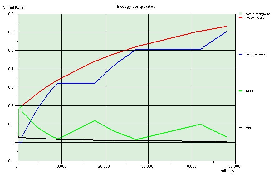
The third step consists of constructing the composite curves. The composite curves play a fundamental role in the pinch method, since the physics and engineering analysis mentioned above are based on these curves.
The hot and cold composite curves are constructed by adding the enthalpies available per temperature level, in the hot and cold streams, respectively. In the figure opposite, the hot composite curve is in red, above the cold composite curve in blue. Their relative positions are characteristic of the system, and the pinches appear at the places where the curves come the closest together (there are two in this example).
The curve showing the difference in Carnot factors, in green on the figure, can be constructed by subtracting the cold composite from the hot composite. The system irreversibilities are exactly equal to the area under this curve.
The pinch points correspond to the most constrained zones of the system. Knowing where they are tells you immediately which streams play a critical role in the global configuration, and which system zones require special care during the design phase.
By displaying the pinch points in a way that is easy to visualize from a physics standpoint, this method provides a valuable guide replacing older heuristic methods that often required numerous iterations.
Based on the results obtained in the previous two steps, process modifications can be considered. Modifications are helpful if you can shift the pinch point(s) and reduce the utility stream, or increase the production of useful energy. Iterations are then performed between the time when the model parameters are reset in the simulator and steps 2 and 3 of the optimization method.
The fourth step consists of matching the streams to construct the heat exchangers. This relatively long and complex step should not be undertaken until the model parameters are deemed satisfactory. The process is facilitated by using the exchange blocks.
For example, the exchanger network obtained to optimize a dual pressure combined cycle is given below.

You can find additional information in the documentation of the optimization method.
