Foundations of the method
If you disregard the relatively complex theory that this method is based on which has been exposed in previous sections (derived from the pinch method with distinction of components and system irreversibilities, Thermoptim optimization method is relatively easy to present and use.
Let us start by saying that this is a variant of the Linnhoff method applied to energy systems. The Linnhoff method is used when designing complex exchanger system with a great many streams, for chemical engineering applications for example.
A relatively complex energy system can have quite a large number of streams that exchange heat, some heating, some cooling. These streams are generally matched in a number of different ways, and selecting the best architecture is not necessarily intuitive, far from it. However, this architecture has a direct effect on internal irreversibilities, and thus on the system's effectiveness. By maximizing the internal regeneration, we obtain the best performance.
To choose a powerful exchanger configuration, thermal integration methods appear to be the best. They also have the advantage of appealing to analysts' physics sense, whereas purely automatic methods requiring working by trial and error.
But their main benefit is that the exchanger system architecture is not defined until after energy consumption is minimized. To optimize the heat exchanges, you simply need to know what streams are involved, without needing to make assumptions about how they are matched. This is a very important feature, as it considerably simplifies the optimization process by making it possible to work in two main phases.
Energy system design tools using these methods are extremely useful for optimization in modern ultra high efficiency power plants or cogeneration units, where pinch analysis is used (in recuperation exchangers, at the water supply, etc.), whereas they did not appear in older plants.
In order to be able to vary the system parameters easily, Thermoptim provides a modeling environment in which the simulation functions and the optimization methods are closely interconnected.
Practically speaking, the method can be broken down into two main phases:
The first phase consists of describing the system without making any assumptions about how the exchangers are matched (this is called a non-constrained system), and seeking to optimize the energy recovered (electric power produced, power cogenerated, etc.) using thermal integration algorithms to make sure there are no temperature incompatibilities. The iterative procedure consists of simulating changes in the key system parameters (flow rates, temperatures, pressure levels) and optimizing the performance, while using the pinch method to make sure that you are not introducing any additional high temperature heat needs and that you are minimizing low temperature discharges. The distinction between component irreversibilities (specific to their own operation) and system irreversibilities (related to the system architecture) will tell you how much freedom you have in terms of design. At this point in the process, the people in charge of optimization and the process designers will exchange information back and forth. One of the advantages of this method is that you can get an idea of the optimization possibilities at any time. All the usual thermal integration graphics tools are accessible, as well as the curve showing the difference in Carnot factors, which is well suited to the problem at hand.
The second phase, once the system is optimized, consists of designing a compatible exchanger configuration (the use of the optimization method ensures that a compatible configuration does exist), by matching and splitting streams as necessary (in series or parallel). Thermoptim proposes exchange blocks so you can define the system progressively in phases, by matching the streams starting at the most restricted areas, namely the pinches. If there are technological or financial issues that make it necessary to choose an exchanger configuration other than the one that gives the best performance, it will become apparent during this phase.
Up to now we assumed that the exchanger system was not known. If it is known, you can obviously use Thermoptim to model and test it. You can compare the initial configuration with the configuration that a non-constrained optimization would have given. It is also possible to preset just some of the exchangers and optimize the rest of the system. Thermoptim will combine the constrained exchangers and the free exchangers, which facilitates the global optimization of the system.
Using the method
The method is carried out in four steps, the first three of which correspond to the first phase presented above, and the last being building the exchangers. Remember that the power of the method is based on the fact that it is not necessary to define the exchanger system beforehand. You build it only once the optimal configuration has been found.
First step
The first step consists of selecting the streams that are to be taken into account by the pinch analysis algorithms. The streams can be grouped into two categories: Hot streams, or availabilities, which must be cooled and that release heat, and cold streams, or needs, which must be heated. The streams are selected from the simulator, and the streams are generally exchange-type processes, or thermocouplers.
To select a stream, open its screen, check the option "pinch method stream" and enter the Tmin value you want to set in the “minimum pinch” field. Thermoptim's method is a variation of the Linnhoff algorithm in which several minimum pinch values can be used, depending on the type of stream. For example, the values can be equal to 16 K for gases, 8 K for streams and 6 K for exchanges resulting in boiling or condensation.
In pinch analysis, it is often better to start by not taking into account the hot and cold utilities, representing the non-predetermined heat sources or sinks. Once the other exchangers have been placed and the internal regeneration has been maximized, you are in a better position to design these utilities.
The thermal integration algorithms work under the standard assumption in exchanger calculations that the heat capacity flow rate of each stream (mCp) is constant and equal to the average value obtained by dividing total enthalpy by the difference between the inlet and outlet temperatures. During the optimization procedure, when you split the streams and determine the minimum pinch again, you will see a slight difference with respect to the results obtained previously. This is because when the stream is split, the enthalpy of the intermediate point calculated precisely by Thermoptim is slightly different from the enthalpy that was used initially, and consequently a small adjustment is necessary.
Second step
Once the streams have been selected, the second step, called "pinch minimization", is used to calculate the minimum heating loads to be supplied by the utilities. The pinch is minimized by using a variant of Linnhoff's Problem Table Algorithm (PTA). Thermoptim sorts the stream temperatures and builds a table in which the temperature limits are stored in decreasing order. For each temperature interval, it calculates the sum of the enthalpies of hot and cold streams. From this you can deduce the utility requirements. If the internal availabilities are sufficient to satisfy the needs (in other words if the temperature and quantity are sufficient) the utility requirement is equal to zero. If this is not the case, either because there is not a sufficient quantity or because the exergy level is too low, Thermoptim determines the minimum utility required. By accurately determining the minimum utility requirements, this step defines a target that can be used to precisely quantify the difference between the theoretical optimum and the best solution from a technical and financial standpoint.
Third step
The third step consists of constructing the composite curves and exporting the curves from Thermoptim as a text file called ‘cc_gcc.txt" containing the value pairs (T, h) for the different intervals. The composite curves play a fundamental role in the pinch method, since the physics and engineering analysis mentioned above are based on these curves.
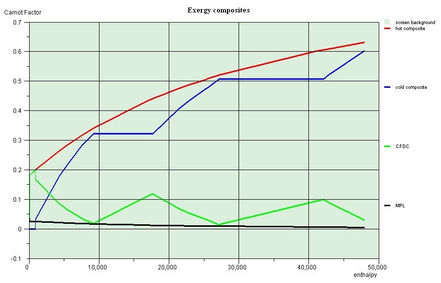
The hot and cold composite curves are constructed by adding the enthalpies available per temperature level, in the hot and cold streams, respectively. In the figure opposite, the hot composite curve is in red, above the cold composite curve in blue. Their relative positions are characteristic of the system, and the pinches appear at the places where the curves come the closest together (there are two in this example).
The curve showing the difference in Carnot factors, in green on the figure, can be constructed by subtracting the cold composite from the hot composite. The system irreversibilities are exactly equal to the area under this curve. You can also see a black curve, called the Locus of Minimum Pinches, which is used in the optimization method to distinguish two different types of irreversibilities. The first, called component irreversibilities, are characteristic of component operation, while the second, called system irreversibilities, are specific to the system architecture. Distinguishing between the two types of irreversibilities shows how much system-specific freedom you have to work around particular technological constraints, with no detriment in terms of energy.
The pinch points correspond to the most constrained zones of the system. Knowing where they are tells you immediately which streams play a critical role in the global configuration, and which system zones require special care during the design phase.
By displaying the pinch points in a way that is easy to visualize from a physics standpoint, this method provides a valuable guide replacing older heuristic methods that often required numerous iterations.
Based on the results obtained in the previous two steps, process modifications can be considered. Modifications are helpful if you can shift the pinch point(s) and reduce the utility stream, or increase the production of useful energy. Iterations are then performed between the time when the model parameters are reset in the simulator and steps 2 and 3 of the optimization method.
Fourth step
The fourth step consists of matching the streams to construct the heat exchangers. This relatively long and complex step should not be undertaken until the model parameters are deemed satisfactory. The process is facilitated by using the exchange blocks presented below
References
For more information, please see the documents listed in the references, in particular chapter 22 of the book "Energy Systems", which presents the method and looks at a step-by-step example of a heat recovery steam generator (HRSG) like those used to produce steam in combined cycles or in cogeneration plants. In an HRSG, the steam is produced at 2 to 4 pressure levels, which can be selected freely within certain limits. The steam properties are highly non-linear functions of temperature and pressure, the steam flow rates can vary depending on the operating conditions, and the heat exchanger matching possibilities are numerous. Moreover, whereas conventional boilers must satisfy exhaust temperature constraints, and therefore cannot be totally optimized from a thermal standpoint, HRSGs must satisfy pinch point constrains, so that when optimizing, you must take into account both the steam cycle and the heat exchange with the exhaust.
Chapter 22 of the book Energy Systems is devoted to tjis issue.
GICQUEL R., Energy Systems: A New Approach to Engineering Thermodynamics, January 2012, CRC Press, ISBN-13: 978-0415685009
GICQUEL R., Méthode d’optimisation systémique basée sur l’intégration thermique par extension de la méthode du pincement : application à la cogénération avec production de vapeur, Revue Générale de Thermique, tome 34, n° 405, octobre 1995.
GICQUEL R., MODICS. Généralisation de la méthode d’optimisation systémique aux systèmes thermiques avec échangeurs imposés, Revue Générale de Thermique, tome 35, p. 423-433, 1996.
LEIDE B., GICQUEL R., Systemic approach applied to dual pression HRSG, International Gas Turbine & Aeroengine Congress and Exhibition, Orlando, Florida, 2-5 June 1997
LINNHOFF B., Use pinch analysis to knock down capital costs and emissions, Chemical Engineering Progress, august 1994, pp. 32 – 57
LINNHOFF B., HINDMARSH E., The pinch design method for heat exchanger networks, Chemical Engineering Sc., Vol. 38, n° 5, pp. 745-763, 1983.
LINNHOFF B., User Guide on Process Integration for the Efficient Use of Energy, Pergamon Press, Oxford, 1982.
Implementation in Thermoptim
Caution: only "professional" and "industrial" Thermoptim versions provide access to optimization functions.
All of the functions specific to optimization are accessible from the optimization window (Special menu). They work in close coordination with the simulator, so you can easily modify the system parameters.
Optimization screen
To get access to the optimization screen, type Ctrl M or select "Optimization tools" in the "Special" menu. The optimization screen is the following:
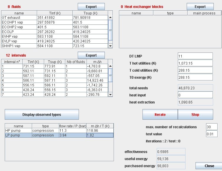
It is comprised of four main tables:
the fluid table contains all the exchange fluids in which the "pinch method fluid" checkbox is selected. These are the fluids which are processed by the variant of the Problem Table Algorithm implemented in Thermoptim.
the interval table contains the list of the intervals which are built by the PTA variant. It will be explained in more detail later
the heat exchanger block table contains the exchange blocks which can be defined in order to facilitate fluid matching in heat exchangers ;
The observed type table shows the points or processes whose "observed" field was checked. These are usually items that are modified during the optimization process, before making a recalculation.
In the lower right part of the screen appear several fields, five of which are editable:
DT MPL is the minimum pinch value used for plotting the minimum pinch locus. By default it is set to 11 K
Thot utilities is the temperature used to plot the hot utilities target (heat input requirements). By default it is set to 1000 K. It should be greater than the existing fluid temperatures.
Tcold utilities is the temperature used to plot the cold utilities target (heat extraction requirements). By default it is set to 300 K. It should be lower than the existing fluid temperatures.
T0 exergy is the value used for temperature reference in exergy calculations. By default it is set to 273.15 K (0 °C)
total needs represents the sum of all the enthalpies of the cold fluids
heat input is the value of the additional heat which may have to be provided to the hot fluids if the total needs exceed the heat available when the pinches are taken into account. This value is also often referred to as the "energy target".
heat extraction represents the value of the heat which must be extracted from the system by cold utilities. It should be noted that the existence of pinch points explains that, as shown above, there may be at the same time a need for a heat input (at high temperature) and for a heat extraction (at low temperature).
Two buttons "Iterate" and "Stop" to automate the recalculation based on certain criteria. Both fields below are used to define the maximum number of iterations and the desired accuracy. The accuracy test is done on the sum Delta of absolute values of differences between the energies of different types (useful, other and purchased) obtained for two successive recalculations. If Delta is less than the specified accuracy, recalculation is stopped.
Once these parameters are specified, the recalculation is initiated by clicking button "Iterate". The results are summarized below, in the form of valuesof efficiency, useful and purchased energy , the number of iterations, and the test value. The "Stop" button allows one to stop the iterations if necessary. Before using this advanced feature, it is preferable to properly ensure that the model is valid and that the calculations converge, and to save it.
Fluid table
When you double-click on one of the fluids listed in the fluid table, the following frame appears:
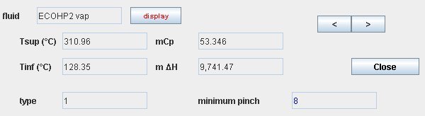
It summarizes the data which is processed by the PTA and cannot be directly modified by the user, as it is built from the corresponding process which can be shown by clicking on the "display" button.
Intervals
Interval analysis plays an important role in pinch methods, as they allow to understand how the different fluids are distributed. In particular the analysis of the intervals around the pinch points is of basic importance for efficiently matching fluids in heat exchangers. The intervals can be displayed either from the optimization frame, or from the charts themselves, by double-clicking on the diagram: the corresponding temperature is calculated, and the interval in which it is contained is displayed.
When you double-click on one of the lines of the interval table, the following screen appears:
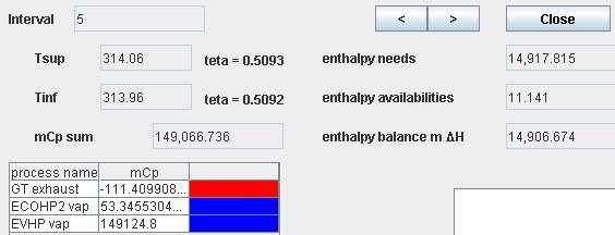
In the upper left zone are shown the number of the interval, its temperature limits Tsup and Tinf and their equivalents in teta Carnot factor, as well as the algebraic sum of the thermal capacity flow rates mCp of the different fluids which are contained in the interval.
On the right are indicated the sum of the enthalpy needs and availabilities in the interval and the corresponding enthalpy balance.
The list of the fluids which are located in or cross the interval is displayed in the table with the value of their thermal capacity flow rate mCp. If you double-click on one of them, the corresponding process frame is shown.
The color associated with the fluid is red in the case of availability (fluid which cools), and blue in the case of a need (fluid which warms).
Exchange blocks
Heat exchanger blocks have been introduced in order to facilitate heat exchanger matching when a main process exchanges heat with several processes as for instance when one seeks to recover heat from gas turbine flue gases. In such a case the main hot fluid has to be divided (in series and/or in parallel) in several subprocesses to be matched with the different cold fluids.
The role of the heat exchanger blocks is to provide assistance for dividing the main exchange process: one begins by grouping the fluids to be matched in blocks which are balanced at the enthalpy level ; in a second step, the choice is made between series or parallel matching, and lastly the main fluid can be further divided. Only exchange processes included in the optimization method can be matched in exchange blocks: thermocouplers must be separately matched directly (this choice was made taking into account the peculiarities of thermocouplers, which are mostly defined in external components).
Heat exchanger blocks are only used as part of the optimization method. They differ from the classical heat exchangers which are accessible from the main project screen. When the heat exchanger blocks have been defined, it is possible to divide the main process in as many subprocesses as required. Once this division is made, the classical heat exchangers can be easily built from the block frame.
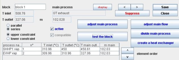
The name of the block appears in the upper left zone. On its right is the double-clickable field defining the main process (here "GT exhaust"), which may be displayed by clicking on the red button "display".
Below the block and main process names are located checkboxes which allow one to characterize the block: its elements may be matched in series or in parallel, and the block may be "upper" or "lower constraint" as explained below.
The block may be "active" or not: only those blocks which are active are taken into account in the optimization method for the mixed problem when some heat exchangers are set. If the block is balanced at the enthalpy level and the temperatures of the different fluids comply with the pinch constraints, the block is "compatible".
On the lower left part of the frame is a table where are listed the different fluids which are to be matched with the main process. They can be added either by double-clicking in the table headband or by clicking on the button "add an element". They can be removed by clicking on the button "suppress an element". The fluid order may be modified by selecting one of them and shifting it using the two arrows on the right of the table. If you double-click in the table, the process corresponding to the fluid is shown.
Five blue buttons allow one to use the block:
the button named "adjust main process" allows you to adjust the block enthalpy balance by modifying the inlet or outlet temperature of the main process. Thermoptim calculates the total enthalpy corresponding to the different elements which have been selected and sets that of the main vein to that value. If the "upper constraint" is selected, the minimum temperature of the vein is modified (the outlet one for a hot fluid, and the inlet one for a cold one). If the "lower constraint" is selected, this is done conversely.
the button "adjust the main flow" allows you to balance the enthalpy balance of the block by changing the flow of the main process;
The button named "test the block" allows you to check the block consistency. Before activating it, it is necessary that the main process be adjusted by clicking on the previous button. Thermoptim checks the temperature compatibility between the main vein and the different block elements.
Once a block is valid, it is possible to divide it into smaller blocks matching a part of the main vein and one of each block elements. If the "series" checkbox is selected, the main vein is divided in series into as many parts as there are block elements, of the same flow rate as the main vein, the intermediate temperatures being calculated. If the "parallel" checkbox is selected, the main vein is divided in parallel into as many branches as there are block elements, of the same temperatures as the main vein, their flow rate being calculated proportionally to the enthalpy of the divided block. Furthermore, you can ask Thermoptim to automatically build the divider and the mixer which connect the main vein divided branches. Thermoptim automatically names the new types which it creates, adding _0, _1... to the existing names, except for the mixer (MIX_xxx) and the divider (DIV_xxx). If a type of that name already exists, it is modified.
the fifth button named "create a heat exchanger" allows you to automatically start building the classical heat exchanger corresponding to a block comprised of a single element. If the two fluids of the block are already connected in an existing heat exchanger, a message warns you. In any case, the heat exchanger screen is shown. If it is created, you have to finish to define it by selecting the constraints and the type of calculation before calculating it. By default, the heat exchanger type is created of the counterflow type, but you can change it if you wish to do so.

Optimization menus
Currently the following menus are available:
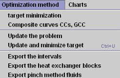
target minimization corresponds to the shifted temperature PTA
composite curves CCs, GCC builds up the composite curves
update the problem updates the optimization elements from the process table
update and minimize the target combines the third and first items
Export the intervals creates a text file named "interv.txt" in subdirectory "pinch" containing all the information on the intervals
Export the heat exchanger blocks creates a text file named " HXblock.txt" in subdirectory "pinch" containing all the information on the heat exchanger blocks, as well as preliminary computations of the exchanger characteristics (effectiveness, NTU, LMTD, UA value)
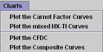
plot the Carnot Factor curves plots the exergy composite curves
plot the mixed HX-TI Curves plots the composite curves obtained when part of the heat exchanger network is set.
plot CFDC plots only the Carnot Factor Difference Curve
plot grand composite curves plots these curves
The two latter menu items are enabled only when either the Carnot Factor or the mixed HX-TI curves have been calculated.
