Plot of cycles in the (h, ln(P)) chart
Introduction
We now have almost all the elements to calculate the performance of the cycles of the steam power plant, the gas turbine and the refrigeration machine, by plotting them in the (h, ln (P)) charts which will provide us with the values of the enthalpies put in play. We will do this after clarifying a few points, notably concerning the calculation of efficiencies.
We will only present a simplified version of the gas turbine cycle where combustion is replaced by heating, the estimation of the thermodynamic properties of the combustion products requiring special precautions. More realistic models taking combustion into account will be presented in another course.
In practical terms, the activities proposed in this section should be done by hand, with charts on paper. These can either be obtained commercially or in specialized books or printed directly from Thermoptim, but their accuracy is not very high. For the gas (h, ln (P)) charts, this will probably be the only solution, as this type of chart is seldom used.
Concept of isentropic efficiency
To determine the performance of the cycles, we will first assume that compressions and expansions are perfect, that is to say follow reversible adiabatic, then we will indicate how to take into account the irreversibilities in these machines.
Recall that we have indicated that it is possible to characterize a real process by introducing an imperfection factor, often called effectiveness or efficiency, which expresses its performance compared to that of the reference process.
The concept of isentropic efficiency makes it possible to characterize the performances of compressors and turbines which, in reality, are not perfect, so that compression and expansion follow non-reversible adiabatic.
In the case of a compressor, the isentropic efficiency is defined as the ratio of the work of the reversible compression to the actual work, and in the case of a turbine as the ratio of the actual work to the work of the reversible expansion. It should be noted that η is less than or equal to 1 for compression as for expansion (Figure below).
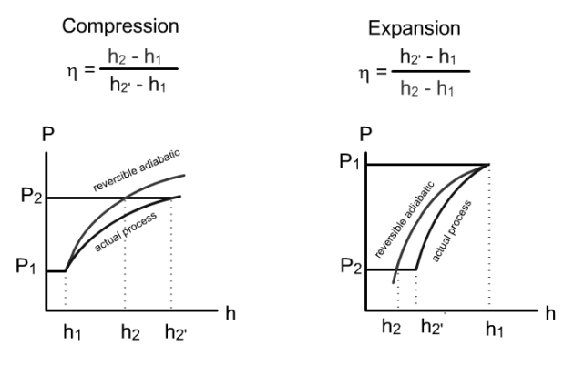
To remember its definition, it suffices to remember that
 is always equal to the smallest work divided by the largest work, and that irreversibilities have the effect of increasing the compression work and reducing the expansion work.
The values of these efficiencies, which depend very much on the technologies used, are typically between 0.75 and 0.9 in current applications.
Self-assessment activity
This self-assessment activity will allow you to test your knowledge on these topics:
Notion of cycle overall efficiency
It may be helpful at this stage to specify what is meant by the notion of efficiency or effectiveness, although we have already used it several times.
Let us in particular specify what is covered by these notions used to characterize the overall performance of a cycle, when establishing its energy balance. For a heat engine which converts heat into mechanical power, it is the ratio of the power output to the heat supplied to the machine:

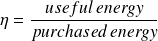
In more general terms, when dealing with relatively complex cycles, one is led to adopt a broader definition of efficiency or effectiveness: it is the ratio of the useful energy effect to the purchased energy put in.
- the purchased energy generally represents the sum of all the energies which one had to supply to the cycle coming from surroundings;
- the useful energy represents the net balance of the useful energies of the cycle, that is to say the absolute value of the algebraic sum of the energies produced and consumed within it participating in the useful energy effect.
Note that the result obtained depends directly on the way in which the boundaries of the cycle are chosen. If we refer to the two examples given above, the work supplied to the pump of a steam plant cycle will be counted as useful energy if we adopt the usual boundary identified by the letter A in Figure below, and as purchased energy if we retain the boundary identified by the letter B.
This expanded definition of efficiency or effectiveness has the advantage of remaining valid for both power cycles and for refrigeration cycles. In the latter case however, we no longer speak of efficiency because its value generally becomes greater than 1, but rather of COefficient of Performance COP.
Self-assessment activity
This self-assessment activity will allow you to test your knowledge on these topics:
Steam power plant
We will now explain how to draw in the (h, ln (P)) chart the steam power plant.
Perfect cycle
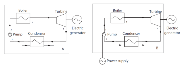
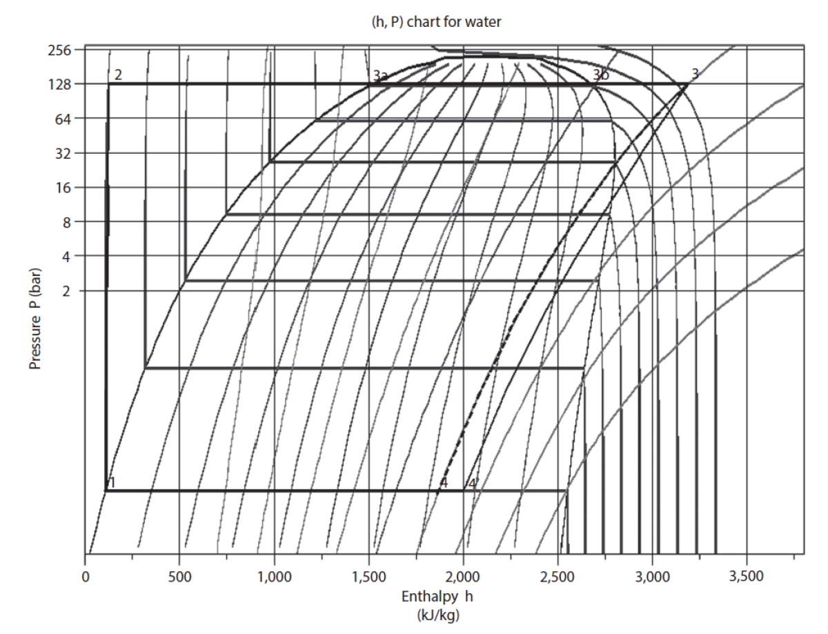
At the condenser outlet (point 1, Figure 2.8), water is in the liquid state at a temperature of about 27 °C, under low pressure (0.0356 bar). In the figure below, the point is easy to find, at the intersection of the isotherm T = 27 °C and the saturation curve.

The pump compresses water at about 128 bar, which represents a significant compression ratio (around 3600).
Temperature T remaining approximately constant during compression (1-2), point 2 is located at the intersection of the isotherm T = 27 °C and the isobar P = 128 bar (ordinate 128 bar).
The pressurized water is then heated at high temperature in the boiler, heating comprising the following three steps:
liquid heating from 27 °C to about 330 °C, saturation temperature at 128 bar, just above isotherm T = 327 °C: process (2-3a). Point 3a lies on the vaporization curve of the same isobaric curve;
vaporization at constant temperature 330 °C: process (3a-3b). Vaporization being carried out at constant pressure and temperature, it results on the chart in a horizontal segment 3a-3b. Point 3b is therefore on the descending branch of the vaporization curve, or dew point curve, at its intersection with the horizontal line of pressure 128 bar;
superheating from 330 °C to 447 °C, process (3b-3). Point 3 is still assumed to be the same pressure, but at a temperature T3 of 447 °C. It is thus at the intersection of the horizontal P = 128 bar and the isotherm T = 447 °C.
Point 3 is also on a concave curve inclined downwards corresponding to a reversible adiabatic.
Process (3-4) is a reversible adiabatic expansion from 128 bar to 0.0356 bar. The point being in the mixed zone, the latter is within isotherm T = 27 °C. Point 4 is at the intersection of the concave curve inclined downwards and this isotherm. Quality x is between 0.7 and 0.8. Linear interpolation allows us to estimate its value, equal to 0.72.
The enthalpies of the points can be read directly by projecting these points on the x-axis, and the energies involved can be easily deducted. This allows us in particular to determine the cycle efficiency. Table 3.1 provides these values.
Note that reading the compression work in this chart is very imprecise and it is best estimated from the integration of δ
 = v dP, very easy to make, v being constant. It is therefore Δh = v ΔP, P being expressed in Pa, v in m3/kg and h in J.
The figure below shows the cycle in the chart, the points being connected.
The efficiency here is the ratio of the mechanical work produced (1306 kW), to the heat supplied by the boiler (h3 – h2 = 3063 kW), as shown in Table 3.1.
Process |
| Q (kW) |
|
(1-2) | 13 | 13 | |
(2-3a) | 1398 | 1398 | |
(3a-3b) | 1148 | 1148 | |
(3b-3) | 517 | 517 | |
(3-4) | -1319 | -1319 | |
(4-1) | -1757 | -1757 | |
Cycle | -1306 | 1306 | |
Efficiency | 42.64% |


Cycle taking into account deviations from reference processes
In reality, the turbine is not perfect, and expansion follows an irreversible adiabatic. It is customary to characterize the actual process by its isentropic efficiency
, defined in the case of a turbine as the ratio of actual work to the reversible expansion work. Its value is typically about 0.85 to 0.9 in current applications.
To find the actual point 4', we first determine the value of the perfect machine work
 , then we multiply it by
, which gives the value of actual work
, then we multiply it by
, which gives the value of actual work
The enthalpy of point 4 is equal to that of point 3 minus
.
In this case, taking
= 0.9, we have:
= h3 – h4 = 1319 kJ/kg/K
=
 = 0.9 x 1319 = 1187
h4' = 3199 – 1187 = 2002 kJ/kg/K
Point 4', which is still in the liquid-vapor equilibrium zone, is thus on isobar P = 0.0356 bar, i.e. on isotherm T = 27 °C with abscissa h = 2002 kJ/kg/K. The figure below shows the new look of the cycle (the previous cycle is plotted in dashed line).
The increase in the quality at the end of expansion is favorable on the one hand to the prolongation of the life of the turbine blades, for which the liquid droplets constitute formidable abrasives, and on the other hand to the isentropic efficiency, which drops when the quality decreases.
Here we have not considered the pressure drops in heat exchangers. It would of course be possible to do so by operating on the same principle as described, and changing the pressure between the inlets and outlets of heat exchangers.
As shown in this example, the representation of the cycle in the (h, ln(P)) chart is very easy to understand: the heat exchanges, almost isobaric, correspond to horizontal segments, and the compression and expansion are reversible adiabatic, less steep as they are located far from the liquid zone.
Gas turbine
We are now going to construct the gas turbine cycle plot in the air (h,ln(P)) chart.
Perfect cycle
The gas turbine draws 1 kg/s of air at 25 °C and 1 bar and compresses it to 16 bar in a perfect compressor. This air is brought to the temperature of 1065 °C in the combustion chamber, and then expanded in a perfect turbine.
We assume initially that compressions and expansions are perfect, that is to say they follow the reversible adiabatic, then we shall explain how to take into account the irreversibilities in these machines.
In the (h, ln (P)) chart in the figure, point 1 is on the x-axis, at the intersection with the isotherm T = 25 °C (h = 0). Perfect compression along the reversible adiabatic leads to point 2, the intersection of this curve and the horizontal P = 16 bar. The enthalpy can be read on the abscissa and is h = 360 kJ/kg.
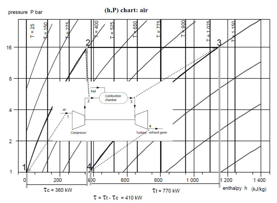
The heating in the combustion chamber leads to point 3, at the intersection of the isobar P = 16 bar and the isotherm T = 1065 °C (h = 1140 kJ/kg).
Process (3-4) is a reversible adiabatic expansion from 16 bar to 1 bar. Point 4 is therefore at the intersection of the reversible adiabatic and the abscissa axis (h = 375 kJ/kg).
This chart helps to understand why the gas turbine can operate: the higher the temperature, the less steep the slopes of the reversible adiabatics, and therefore the greater the energy involved in the process, for a given pressure ratio: the enthalpy variation (3-4) increases much faster than the compression work (1-2). We therefore have an interest in working at P and T as large as possible.
For the selected setting, the compression work
 at 1 bar and 25 °C is more than twice smaller than the expansion work
 at 16 bar and 1065 °C.
We also understand why the performance of the machine depends very much on the ambient air temperature: the lower it is, the steeper the slope of the reversible adiabatic and therefore the lower the compression work.
Point | Flow-rate (kg/s) | h (kJ/kg) |
1 | 1 | 0 |
2 | 1 | 360 |
3 | 1 | 1140 |
4 | 1 | 370 |
The useful energy is the absolute value of the algebraic sum of the work supplied to the compressor and produced by the turbine (410 kW), and the purchased energy is the heat supplied in the combustion chamber (h3 – h2 = 780 kW). The efficiency is deduced from this, as shown in the table below.
Process |
| Q (kW) |
|
(1-2) | 360 | 360 | |
(2-3) | 780 | 780 | |
(3-4) | - 770 | -770 | |
Exhaust | |||
Cycle | - 410 | 780 | |
Efficiency | 52.60% |
The turbomachines having been assumed to be perfect, the efficiency is very high.
Cycle taking into account deviations from reference processes
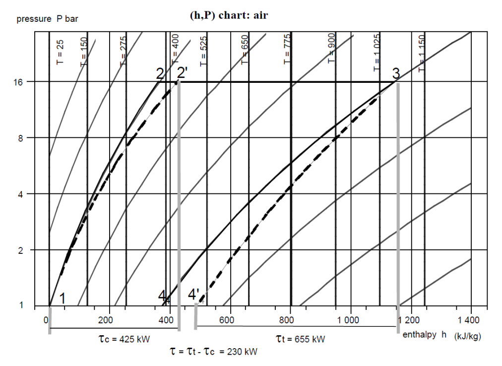
In reality, the compressor and the turbine are not perfect, and compression and expansion follow non-reversible adiabatic. As we explained previously, the real process is characterized by an isentropic efficiency
, defined in the case of the compressor as the ratio of the reversible compression work to the actual work, and in the case of the turbine as the ratio of the actual work to the reversible expansion work.
To find the actual point 2′, we therefore determine the value of the work
required by the perfect compressor and we divide it by
.
As
= h2' – h1, the enthalpy of point 2' is equal to that of point 1 plus
.
In the present case, taking
= 0.85, we have:
= h2 – h1 = 360 kJ/kg
=
/
= 360/0,85 = 424
h2' = 424 kJ/kg
To find the actual point 4', we determine the value of the work
delivered by the perfect turbine and we multiply it by
, which gives the value of the actual work
.
As
= h3 - h4', the enthalpy of point 4' is equal to that of point 3 minus
.
In the present case, taking
= 0,85, we have:
= h3 – h4 = 765 kJ/kg
=
= 0.85 . 765 = 654
h4' = 1140 – 654 = 486 kJ/kg
The figure below shows the new appearance of the cycle (with dashes, the previous cycle being shown in solid lines). The efficiency drops considerably (it is 32% instead of 52%), because the net work, equal to the difference in absolute value between the work of expansion and that of compression, is greatly reduced. The compression work increased by 65 kW, but above all the expansion work fell by 115 kW, the total loss being 180 kW.
Refrigeration machine
Let us now plot the refrigeration machine cycle in the R134a (h, ln(P)) chart.
Perfect cycle
In accordance with the rapid analysis that we made of the saturation pressure curve of R134a, the evaporation pressure of the R134a refrigeration compression cycle must be less than 2.1 bar, and its condensation pressure greater than 8.8 bar. We will retain 1.78 bar and 12 bar so that the temperature difference with the hot and cold sources is sufficient.
At the evaporator outlet, a flow rate m = 1 g/s of fluid is fully vaporized and thus point 1 (Figure below) is located at the intersection of the saturation curve and the isobar P = 1.78 bar, or, equivalently, the isotherm T = - 13 °C.
It is then compressed at 12 bar along a reversible adiabatic.
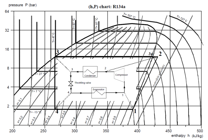
Point 1 being located approximately one third of the distance between two reversible adiabatics on the chart, it is possible, by linear interpolation, to determine point 2 on isobar P = 12 bar, between these two curves.
The refrigerant cooling in the condenser by exchange with outside air comprises two stages: de-superheating (2-3a) in the vapor zone followed by condensation along the horizontal line segment (3a-3). Points 3a and 3 lie at the intersection of the saturation curve and the isobar P = 12 bar, or, equivalently, the isotherm T = 47 °C. Point 3a is located on the right, at the limit of the vapor zone, and point 3 on the left, at the limit of the liquid zone.
Expansion without work, and therefore an isenthalpic process, corresponds to the vertical segment (3-4), point 4 being located on the isobar P = 1.78 bar, or, equivalently, the isotherm T = - 13 °C, at abscissa h = h3. Its quality reads directly from the corresponding iso-quality: it is x = 0.4.
Point | Flow-rate (kg/s) | h (kJ/kg) |
1 | 1 | 391 |
2 | 1 | 430 |
3a | 1 | 422 |
3 | 1 | 266 |
4 | 1 | 266 |
The energies put into play can easily be determined by projecting these points on the x-axis. This allows us in particular to calculate the coefficient of performance COP of the cycle, defined as the ratio of the useful effect (the heat extracted at the evaporator) to the purchased energy (here the compressor work).
The useful energy is the heat extracted from the evaporator (125 kW), and the purchased work energy supplied to the compressor (40 kW). The ratio of the two, equal to 3.14, being greater than 1, the efficiency term is no longer suitable. We talk about the COefficient of Performance (COP) of the cycle. The table below provides these values.
Process |
| Q (kW) |
|
(1-2) | 40 | 40 | |
(2-3a) | -8 | -8 | |
(3a-3) | -157 | -157 | |
(3-4) | |||
(4-1) | 125 | 125 | |
Cycle | 40 | -40 | |
COP | 3.12 |
Cycle taking into account deviations from reference processes
This cycle differs from that of a real machine on several points:
the actual compression is not perfect, so that the compression work is higher than that which would lead to reversible adiabatic;
to prevent aspiration of liquid into the compressor, which could deteriorate it as the liquid is incompressible, the gas is superheated by a few degrees (typically 5 °C) above the saturation temperature before entering the compressor;
before entering the throttling valve, the liquid is sub-cooled by a few degrees (typically 5 °C), as this first ensures that this device is not supplied with vapor, and second increases the refrigerator performance.
Here we can also characterize the actual compression by an isentropic efficiency, defined as the ratio of the work of the reversible compression to real work.
To find the actual point 2', we determine the value of work
in the perfect machine, then divide it by
, which gives the value of actual work
.
The enthalpy of point 2' is equal to that of point 1 plus
.
In this case, taking
= 0.75, we have:
= h2 – h1 = 40 kJ/kg/K
=
/
= 40/0.75 = 53
h2' = 391 + 53 = 444 kJ/kg/K
The cycle changed to reflect superheating, subcooling and compressor irreversibilities is shown in the figure below (the previous cycle is plotted in dashed line).
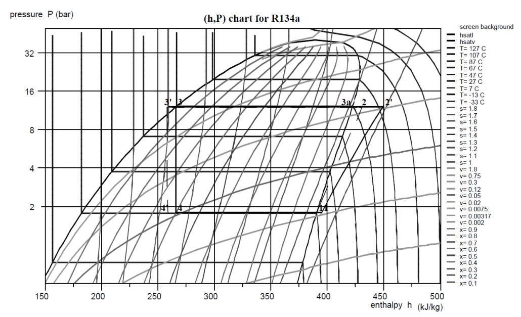
The COP of the machine is of course changed: it drops to 2.57 because of the compressor irreversibilities.
The relevance of sub-cooling can easily be shown in the (h, ln (P)) chart because, for the same compression work, the COP increases as the magnitude of the sub-cooling grows. It is however limited by the need for a coolant.
We did not consider pressure drops in the exchangers. It would of course be possible to do so.
Sself-assessment activities
We will frequently use two concepts which must be well understood, that of isentropic efficiency and overall cycle efficiency.
These self-assessment activities will allow you to test your knowledge on these topics:
Identification of a steam plant cycle in a (h, ln (P)) chart, ddi
Identification of a gas turbine cycle in a (h, ln (P)) chart, ddi
Identification of a refrigeration cycle in a (h, ln (P)) chart, ddi
