Introduction
Guided exploration (OPT-1) has shown you how the pinch method can be applied to optimize a heating network.
The objective of this exploration (DTNN-2) is to explain how to determine the exchange surfaces by using the technological sizing tools of Thermoptim.
Finally, you will study how to obtain the exergy balances of the initial network and the optimized one using their productive structures.
We will operate here in two steps:- sizing of heat exchangers
- determination of the exergy balances of the initial and optimized networks
Brief presentation of the heat network model
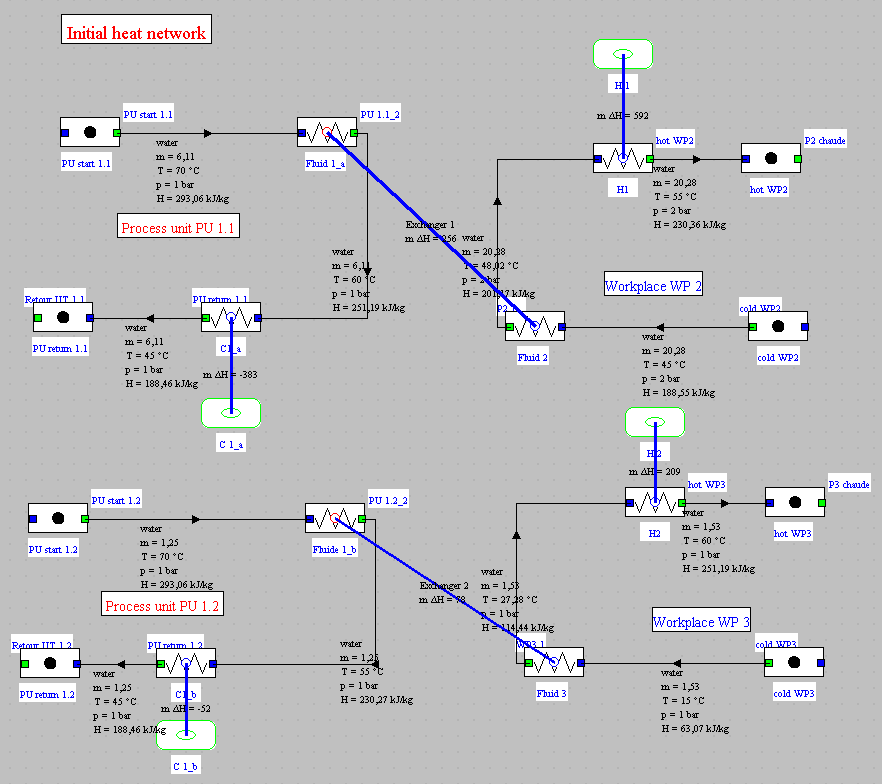
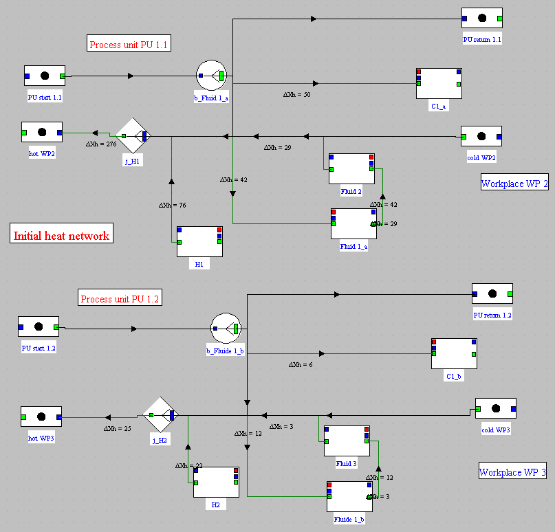
This diagram shows the initial heat network.
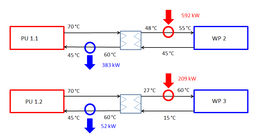
The heating network is used to supply heat to two workplaces:
- workplace WP 2, where 73 m3/h of hot water at 55 °C are needed, which come out at 45 °C
- workplace WP 3, where we need 5.5 m3/h of hot water at 60 °C,
which come out at 15 °C
It can recover heat from two sources:
- the process unit PU 1.1 process unit, where 22 m3/h of hot water at 70 °C are available, which must be cooled to 45 °C
- the process unit PU 1.2, where there is 0.8 m3/h of hot water at
70 °C, which must be cooled to 45 °C
In the existing installation, additional heat is supplied to the two heat utilization circuits.
The total power to be supplied by the hot utilities to the existing installation is 592 + 209 = 801 kW.
As the two hot fluids are not completely cooled, a cooling power of 383 + 53 = 436 kW must be used, which is called cold utilities.
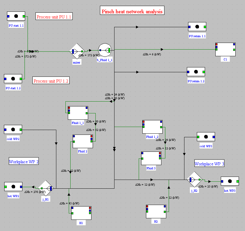
Synoptic view of the optimized installation
The result of the optimization process by the pinch method presented in gided exploration (OPT-1) is given in this synoptic view.
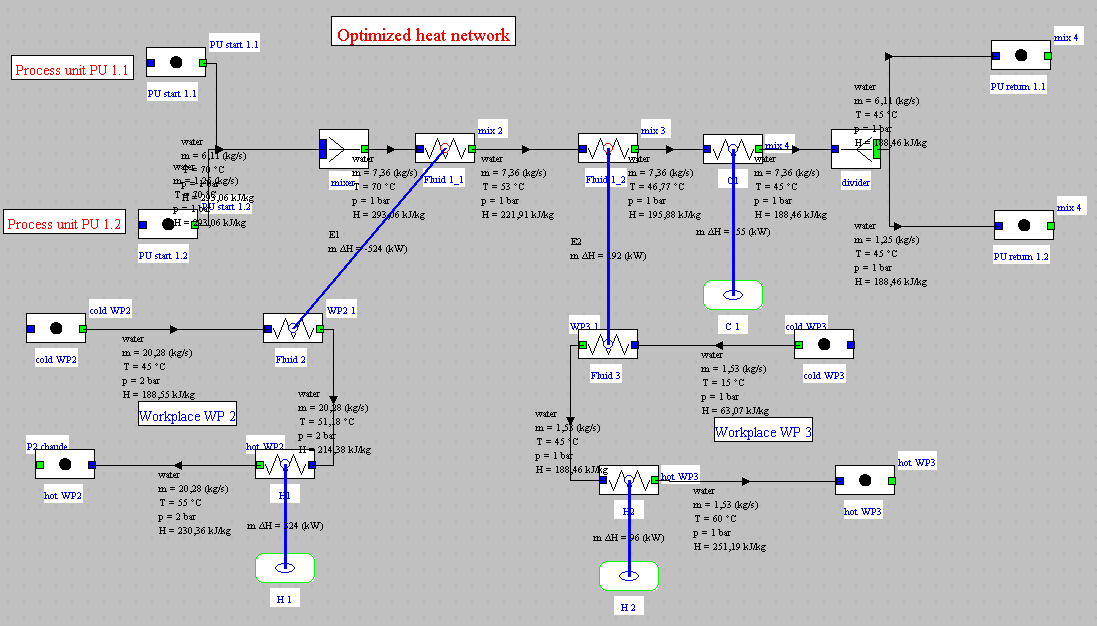
In the following step, we will learn how to size the two heat exchangers E1 and E2.
Determination of the surfaces of exchangers E1 and E2
In this step, we will see how the surfaces of exchangers E1 and E2 can be determined.
The problem arises because the NTU heat exchanger calculation method which is implemented in the Thermoptim core can only determine the product UA of the global heat exchange coefficient U by the surface A of the exchanger, without the two terms being evaluated separately.
To be able to go further and separate these two terms, it is necessary to carry out what we call a technological sizing of the exchanger.
This is a relatively complex problem that you should understand before you can use it. It is presented in this page of the Thermoptim-UNIT portal, which we strongly recommend that you read before anything else.
Versions 2.7 and 2.8 of Thermoptim allow you to perform technological sizing and off-design studies. For this, they introduce screens complementary to those which allow the usual phenomenological modeling to be carried out.
They define the geometric characteristics representative of the different technologies used, as well as the parameters necessary for calculating their performance. For a given component, they obviously depend on the type of technology chosen.
To be able to size an exchanger, that is to say calculate its surface, it is necessary on the one hand to choose its geometric configuration, and on the other hand to calculate U, which depends on this configuration, on the thermophysical properties of fluids, and on the operating conditions.
Let us recall that the approach that we adopted in Thermoptim is not conventional, but that it is consistent with other approaches used in heat exchangers, and proves to be quite fruitful for the study of complex systems: a heat exchanger ensures the coupling between two "exchange" processes, one representing the hot fluid which cools, and the other the cold fluid which heats up. As a result, the definition of the flow configurations and of the geometry of the exchanger is done at the level of each process, and not globally.
Loading the model
Click on the following link: Open a file in Thermoptim
You can also:
- either open the "Project files/Example catalog" (CtrlE) and select model m19.1 in Chapter 19 model list.
- or directly open the diagram file (opt1RDC_Ech_en.dia) using the "File/Open" menu from the diagram editor menu, and the project file (opt1RDC_Ech_en.prj) using the "Project files/Load a project " menu from the simulator.
Loading the generic pilot
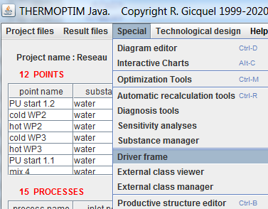
The generic technological design pilot can be loaded from the simulator screen. To do this, activate the "Driver frame" line in the "Special" menu.
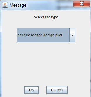
Then select the line "generic techno design pilot" from the list of available drivers, and click "OK".
The pilot screen opens. Click on "Set the technological design screens".
Two rows appear in the table, corresponding to exchangers E1 and E2.
They indicate that they are heat exchangers (HeatEx), and that they are considered as simple exchangers (TechnoHx).
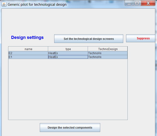
It is possible to change this type by double-clicking on one of the rows. This is what should have been done if one of them was an evaporator or a vaporizer, but this is not the case here.
Technological screens are now created.
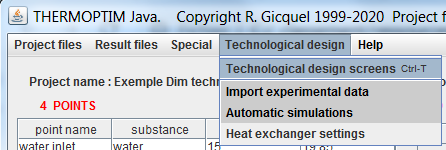
To access them, return to the simulator screen, and activate the line "Technological design screens" in the "Technological design" menu, or type Ctrl T.
The window allowing access to the existing technological design screens is displayed.
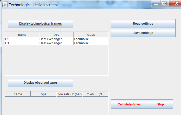
Double-clicking on a table row opens the technological design screen for the selected component.
Technological design screen of an exchanger
Here is the technological design screen of an exchanger set by default.
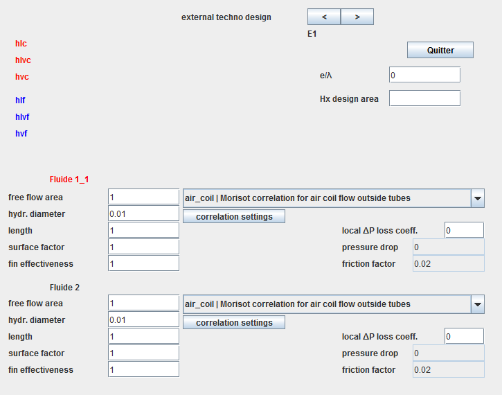
The study of the calculation of the heat exchange coefficients and of the pressure drop shows that, in addition to the surface of the exchanger A, two geometrical quantities play a particularly important role: the passage cross-section assigned to the fluid Ac, and the hydraulic diameter dh. When the heat exchange coefficients of fluids are very different, various devices such as fins are used to compensate for the difference between their values. We then speak of enhanced surfaces, which can be characterized by a surface factor f and a fin effectiveness eta0.
These four parameters are those used in Thermoptim to characterize the heat exchanges for each fluid. We add the length of the exchanger for certain calculations such as pressure drop.
In the technological design screen of the exchangers, the following conventions are adopted:
- the type of configuration (here "air-coil") is selected from a drop-down list
- "free flow area" represents the passage section Ac
- "hydr. diameter" is the usual hydraulic diameter dh
- "length" is the length of the exchanger (used for the calculation of the boiling number Bo and for the calculation of the pressure drop, not yet implemented in the two-phase case)
- "surface factor" is the surface factor f for enhanced surfaces
- "fin effectiveness" is the effectiveness of fins eta0
In our case, there are no fins. The last two parameters are therefore 1.
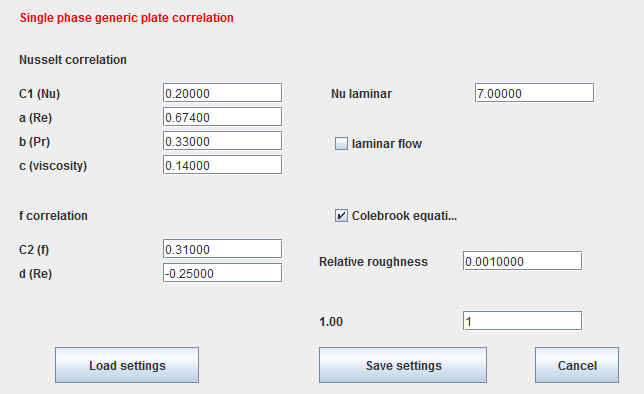
However, the default correlation is not correct. By clicking on "air-coil | Morisot correlation ...", the list of possible choices is displayed. The one that interests us is the last, which corresponds to plate heat exchangers.
The default correlation setting for plate heat exchangers is given below. You can access it by clicking on the technological screen of the exchanger, on the "correlation settings" button located below the correlation type.
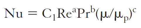
The values of the coefficients C1, a, b and c are those of this classic formula giving Nusselt as a function of Reynolds, Prandtl and viscosity.
If the default values do not suit you, you can modify and save them using the "Save settings" button.
Thermal resistance of the wall
The e/lambda parameter located at the top slightly right of the screen represents the thermal resistance due to the fluid wall (this is the ratio of the thickness of the wall to its thermal conductivity lambda). We will neglect it here.
Setting of exchangers E1 and E2
We will assume that the exchangers used for our optimized installation are 50 cm long plate exchangers whose hydraulic diameter can be estimated at 3.8 mm.
The thermal power of E1 is 524 kW, and that of E2 is 191 kW.
Given that it is a plate exchanger, we will assume that the fluid passage sections are the same for each of the two fluids of the same exchanger, and that they are 0.03 m2 in E1 , and 0.01 m2 in E2.
It only remains to enter these values in the technological screen of each of the two heat exchangers.
To make your task easier, you can simply read these values in the setting files corresponding to these exchangers.
To do this, go to the management window giving access to the technological design screens, and operate as follows for exchanger E1:
- select it in the table
- click on the "Read parameters" button at the top left
- select the file "opt1_echDTNN_E1.par".
All the parameters of the exchanger are then updated.
Do the same for exchanger E2, its setting file being "opt1_echDTNN_E2.par".
Once the technological screens are set, return to the pilot screen.
Then click on "Design the selected components" after selecting the two rows of the table.
Technological screens are calculated. Here is the result for E1.
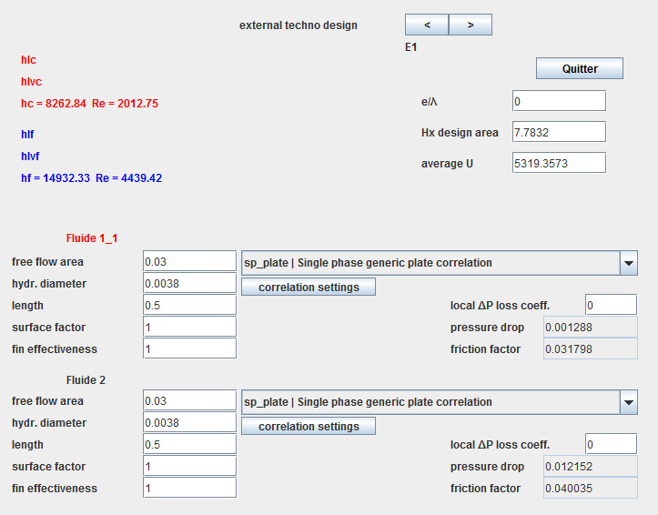
For exchanger E1, the surface determined is equal to 7.78 m2, the overall exchange coefficient being equal to 5319 kW/m2/K.
On the left of the screen are displayed the values of the heat exchange coefficient h within each fluid and those of their Reynolds numbers.
In the case of a single phase fluid like here, only one line is indicated.
The hot fluid appears in red, the cold in blue, according to the usual conventions.
The pressure drop values (in bar) and the friction factor are displayed on the right of the screen, in the setting of each fluid.
Refer to volume 4 of the Thermoptim reference manual for more details.
In the next step, we will compare the exergy balances of the optimized network and the existing one.
Exergy balances of the heat networks
The exergy balances of the optimized network and of the existing network will be calculated using their productive structures.
We assume that you are sufficiently familiar with the concepts used in the study of productive structures, such as those of productive or dissipative unit, junction, branch...
If this is not the case, start by studying the guided exploration BESP-1: Exergy balance and productive structure of a simple steam cycle.
The synoptic view of the initial network is given below.
Loading the model
Click on the following link: Open a file in Thermoptim
You can also:
- either open the "Project files/Example catalog" (CtrlE) and select model m19.2 in Chapter 19 model list.
- or directly open the diagram file (opt1RDC_init_en.dia) using the "File / Open" menu from the diagram editor menu, and the project file (opt1RDC_init_en.prj) using the "Project files/Load a project" menu from the simulator.
If the productive structure editor has not yet been opened, you can access it by pressing Ctrl B or by selecting the "Productive structure editor" line from the "Special" menu of the simulator screen.
You can then open the productive structure file (opt1RDC_init_en.str) using the "File/Open" menu of this editor.
Productive structure of the initial network
Here is the productive structure of the initial network.
For its upper part, it is interpreted as follows: The exergy supplied by the PU 1 is partly transmitted to the fluid 2 in the heat exchanger, partly communicated to the cold utility C1, and partly returned to PU 1.
Fluid 2 receives exergy on the one hand in the heat exchanger, and on the other hand thanks to the hot utility H1.
For its lower part, the analysis is analogous.
Exergy balance of the initial network
The figure below shows the exergy balance of the initial network.
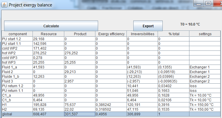
The only information that had to be added to that of the usual Thermoptim project and the production structure are:
- the temperatures of the sources with which the network exchanges heat (we took 10 °C for cold utilities and 150 °C for hot utilities).
- the UPD hot WP2 and hot WP3 have been set as externally valued
(Valuable exergy).
The exergy efficiency is only 49.6%
Loading the optimized model
Click on the following link: Open a file in Thermoptim
You can also:
- either open the "Project files/Example catalog" (CtrlE) and select model m19.3 in Chapter 19 model list.
- or directly open the diagram file (opt1RDC_Ech_en.dia) using the "File/Open" menu from the diagram editor menu, and the project file (opt1RDC_Ech_en.prj) using the "Project files/Load a project " menu from the simulator.
Productive structure of the optimized network
Here is the productive structure of the optimized network.
It is interpreted a little differently from that of the initial network because the two circuits are interconnected. In the upper part, fluid 1 yields exergy to the cold utility C1. In the lower part, it yields exergy to fluids 2 and 3 through the two exchangers E1 and E2.
In the lower part, fluids 2 and 3 receive exergy on the one hand from fluid 1 via the two exchangers E1 and E2, and on the other hand from the hot utilities H1 and H2.
Optimized network exergy balance
The figure below shows the exergy balance of the optimized network.
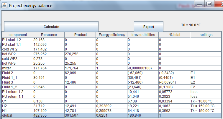
The exergy efficiency has increased, and is now worth 62.5%.
Conclusion
This exploration allowed you to discover how to determine the exchange surfaces by using the technological sizing tools of Thermoptim, thanks to a generic pilot which made it possible to calculate them.
You will find more detailed information on this subject in this page of the Thermoptim-UNIT portal:
Technological design and off-design operation
We also established the exergy balances of the initial and optimized heat networks.
You will find more detailed information on this last subject in the following two pages of the Thermoptim-UNIT portal:
Using the Thermoptim technological sizing screens, it is possible to calculate the overall heat exchange coefficient and to deduce the surface necessary to transmit the desired power.
The concepts underlying these calculations being relatively complex, we recommend that you read the sections relating to exchangers in volume 4 of the Thermoptim reference manual, which are much more detailed than what it is possible to indicate in this guided exploration.
The procedure is as follows: