Introduction

The objective of this exploration is to show you how the pinch method can be applied to optimize a dual pressure combined cycle.

Recall that the OPT-1 guided exploration relates to the optimization of a heat network by the pinch method.

There you will find a detailed presentation of the Thermoptim optimization window and explanations on how to set the fluids that must be taken into account in the optimization process.

It should also be noted that the pinch method is generally used to design a network of heat exchangers between fluids with defined temperatures and flow rates, but that it can also be used to optimize pressure levels and flow rates in combined cycles or cogeneration plants.

This is what this guided exploration will illustrate.

We will start from the setting of the single pressure combined cycle which has been the subject of guided exploration C-M3-V1, and we will seek to improve its performance by adding a second steam cycle to better cool the exhaust gases rejected to the atmosphere.

This will require finding the optimal couple (LP pressure, LP steam flow).

Reminder on the single pressure combined cycle

This synoptic view summarizes the characteristics of the single pressure combined cycle.

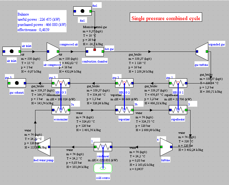
The steam cycle operates with a pressure of 120 bar and a superheating temperature of 520 °C.

The steam flow rate is 74 kg/s.

It cools the gas stream leaving the gas turbine to 164.8 °C, but not lower, so that the overall efficiency of the combined cycle is only 48.6%.

To go further, we will add to this model a second steam cycle at lower pressure.

As we know, the application of the pinch method consists in analyzing the availability and needs of all the fluids involved in the problem.

We build for this the composite curves corresponding to these fluids, which makes it possible to determine where the pinches of the problem are located.

The model does not need to represent the entire existing installation: it is enough for it to show nothing but the fluids involved. This is why it is unnecessary for the heat exchangers to appear at this stage.

We will therefore remove the three existing exchangers, which will also avoid any calculation problem when looking for the optimum.

Initial model

Loading the model

Click on the following link: Open a file in Thermoptim

Diagram editor window display

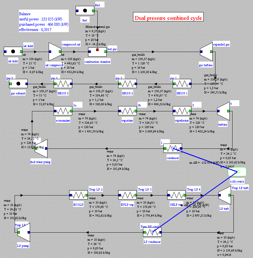
You can see the diagram of the model, with the three fluid circuits involved, their flow rates, and the inlet and outlet temperatures of the different processes.

Parameter retained for optimization by the pinch method

We have set the LP steam cycle for this initial model as follows: pressure equal to 10 bar, flow rate of 10 kg/s and superheating of 50 °C above the saturation temperature.

The isentropic efficiency of the LP turbine was assumed to be identical to that of the HP turbine, namely 0.85.

The exhaust gas temperature to the atmosphere was lowered to 75 °C.

We have also selected the option "pinch method fluid" in all exchange processes except the condensers (exhaust gas stream, economizers, vaporizers, superheaters) by setting the minimum pinches at 16 °C for gases, 8 °C for liquids, and 6 °C for vaporizers.

The combined cycle efficiency now exceeds 50%. Let's see how we can improve it.

Use of optimization tools

Loading the optimization screen

You access the optimization screen, by typing Ctrl M or by selecting the "Optimization Tools" line from the "Special" menu of the simulator screen.

If you can't do it, click this button

This screen has two menus, as you can see for yourself, the "Optimization method" menu and the "Charts" menu.

In practice, however, only two menu lines will be useful:

• Update and minimize target, so that Thermoptim establishes the interval table and calculates the needs for hot and cold utilities after each modification of the model setting
• Plot composite curves to draw these curves which will allow us to visualize the optimization problem

HP flow adjustment

Modify the HP flow in the "economizer" process which is at set flow, reducing its value, for example to 73.5 kg/s, then recalculate the process.

Return to the simulator window, and click several times on "Recalculate" until the balance stabilizes.

Activate again the menu item "Update and minimize target", or type Ctrl U.

A message informs you that an additional 105 kW is required and asks you if you want to save this value.

Answer "OK"

HP flow is still a little too large, but you're getting close to the solution.

Repeat the previous operations, this time entering a value of 73.4 kg/s.

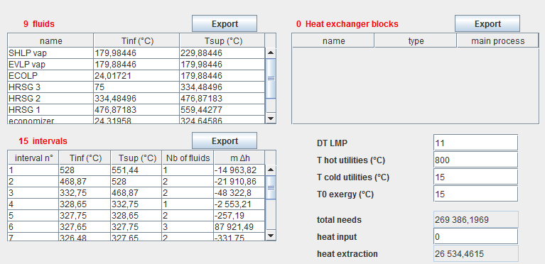
There is no more need for hot utility: pinch is minimized without additional heat.

The optimization screen shows the 9 fluids and 15 intervals.

Plotting composite curves

The composite curves are drawn by activating the Plot composite curves line in the Charts menu.

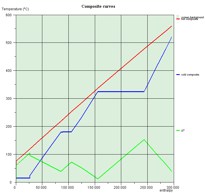
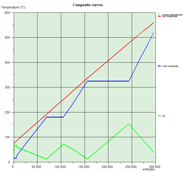
The red curve corresponds to the hot composite, the blue curve to the cold composite, and the green is the difference between the two.

Two pinches appear clearly:

• the upper pinch, at abscissa 85,000 (kW), for a temperature of 180 °C for the cold fluid, and 220 °C for the hot fluid.
• the lower pinch, at the abscissa 1,555,000 (kW), for a temperature of 325 °C for the cold fluid, and 335 °C for the hot fluid.
  

On composite curves, a pinch generally separates two areas:

• the upper zone where the heat requirements of "cold" fluids are greater than the enthalpy available in "hot" fluids, and additional heating is necessary. This zone, deficient in heat, behaves as a heat sink, and is called endothermic zone.
• the lower zone, where the situation is dual from the previous one: "cold" fluids (needs) are unable to absorb all the heat available in "hot" fluids (availability), a surplus having to be evacuated by a complementary cooling fluid. This zone, excess heat, generally behaves like a heat source, and is called exothermic zone;

In a case like this where there are two pinches, the intermediate zone is thermally balanced.

The upper pinch is that which manifests between the HP vaporizer and the gas stream. Its value corresponds to the admissible minimum, and we even had to reduce the flow rate of the initial model to respect the constraints of the problem.

LP flow adjustment

The lower pinch is much larger and can be reduced.

It is enough for that to increase the value of the flow LP in the process "ECOLP", to recalculate it, and to operate as we did when we looked for the good value of the flow HP.

After a few tests, a flow rate of 17.55 kg/s allows the pinch to be reduced below its minimum value.

The new composites that are obtained are given below.

The combined cycle performance has increased, the efficiency now being 51.2%.

However, there is still heat to be removed (5.45 MW as indicated in the optimization window in the "heat extraction" field).

This means that the gas stream cannot be cooled to 75 °C as desired.

Continued optimization

LP pressure adjustment, minimizing the temperature of gas discharge into the atmosphere

Change the LP pressure in the "Tvap LP 1" point at the outlet of the LP pump. The downstream processes "ECOLP", "ELVP vap" and "SHLP" being set as isobaric, the new pressure will propagate up to the inlet of the LP turbine during recalculations.

For example, enter 8 bar as LP pressure in the "Tvap LP 1" point, then recalculate it.

Slightly increase the LP flow value in the "ECOLP" process, for example to 18.4 kg/s, and recalculate it.

Return to the simulator window, and click several times on "Recalculate" until the balance stabilizes.

Activate the menu item Update and minimize target, or type Ctrl U.

The thermal power to be extracted decreases: it is worth 3.3 MW instead of 5.45 MW

LP pressure must therefore be reduced a little more and LP vapor flow must be increased further.

After a certain number of attempts, one obtains a result where there is no need for heat input at high temperature, nor extraction at low temperature. LP pressure is 4 bar, and LP flow 19.84558 kg/s.

We cool the gases to 75 °C, but the performance of the combined cycle has deteriorated: its efficiency is only 48.5%.

This means that this two-stage pressure cycle cannot cool the gases as requested.

If we wanted to do it, we would have to add a third steam cycle.

LP pressure adjustment, maximizing the performance of the combined cycle.

We are resuming the optimization process where we were with LP pressure equal to 10 bar.

The cycle efficiency is 51.21%. Consider the effect of a slight drop in LP pressure.

Now enter 9.5 bar as LP pressure, then recalculate the point "Tvap LP 1".

By operating as above, look for the value of the LP flow rate in the "ECOLP" process which minimizes the lower pinch without adding additional heat. The value of 17.765 kg/s leads to a very slight increase in efficiency, which goes to 51.22%

If you now slightly increase the LP pressure, for example to 10.5 bar and minimize the lower pinch, the efficiency drops to 51.2%.

This means that the optimum is at a LP pressure of less than 9.5 bar.

By continuing the research, we realize that the optimum is very flat and that it is located at a LP pressure of about 9 bar.

Here is the new synoptic view that we obtain.

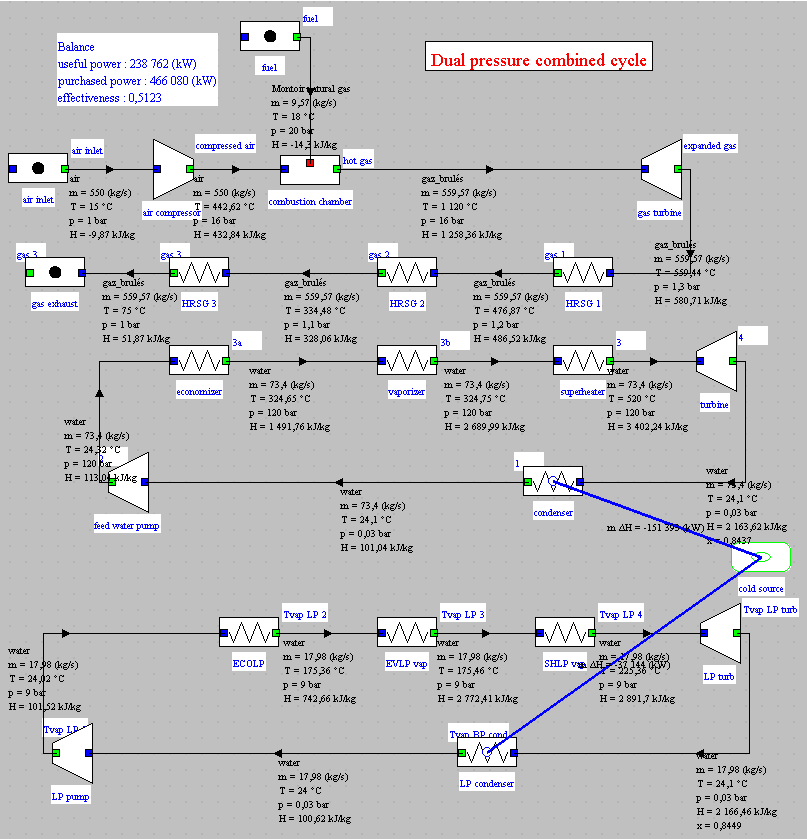
The mechanical power produced is 238,731 MW, whereas before the optimization process it was only 233,855 MW.

The gain is 4.9 MW, or 2%.

In this guided exploration, we were content to seek an optimal setting of the LP steam cycle, considering that the HP cycle was set.

In fact, to go to the end of the process, it would also be necessary to play on the HP pressure and flow, even on the values ​​of the two LP and HP superheating temperatures.

This does not pose any particular methodological problem, but the procedure would of course take longer to implement.

We leave it to you to continue the optimization if you wish.

Access to the optimized model

If you want to load this last model, click on the following link: Open a file in Thermoptim

Conclusion

The pinch method is a very useful guide when trying to optimize a combined cycle with several pressure levels.

As we said, we were content in this guided exploration to seek an optimal parameter setting of the LP steam cycle, by considering that the HP cycle was set.

It would also remain to find the architecture of the heat exchanger network making it possible to achieve this optimum, because in practice at least part of the superheaters and economizers would have to be parallelized.

Thermoptim has the tools to do so, but this goes beyond the scope of this guided exploration.

You will find more detailed information on this subject in the following two pages of the Thermoptim-UNIT portal:

Heat integration or pinch method

Presentation of the Thermoptim optimization method