Introduction
The objective of this exploration (OPT-1) is to show you, in a simple example, how the pinch method can be applied to optimize a heat network.
Note that a second guided exploration (OPT-2) concerns the use of the pinch method to optimize the pressure levels and the flow rates in a dual pressure combined cycle.
We will operate here in two steps:
- identification of the energy target by minimizing the pinch
- construction of the optimized exchanger network
Brief presentation of the heat network model
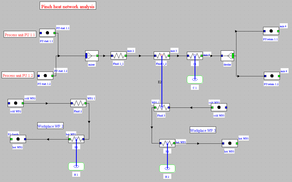
This diagram shows the internal heat network of an agro-food factory that we are trying to optimize using the pinch method.
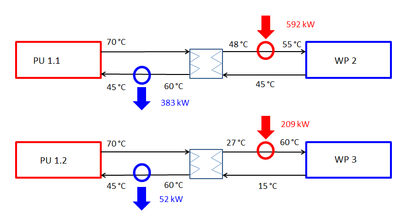
The heating network is used to supply heat to two workplaces:
- workplace WP 2, where 73 m3/h of hot water at 55 °C are needed, which come out at 45 °C
- workplace WP 3, where we need 5.5 m3/h of hot water at 60 °C,
which come out at 15 °C
It can recover heat from two sources:
- the process unit PU 1.1 process unit, where 22 m3/h of hot water at 70 °C are available, which must be cooled to 45 °C
- the process unit PU 1.2, where there is 0.8 m3/h of hot water at
70 °C, which must be cooled to 45 °C
In the existing installation, additional heat is supplied to the two heat utilization circuits.
The total power to be supplied by the hot utilities to the existing installation is 592 + 209 = 801 kW.
As the two hot fluids are not completely cooled, a cooling power of 383 + 53 = 436 kW must be used, which is called cold utilities.
The objective of the study is to try to reduce these two values.
We will start by looking at what improvements can be made without changing the structure of the installation, ie by playing only on heat exchangers and utilities.
We will therefore begin by studying a Thermoptim model of the existing network.
It is only in a third step that we will use the pinch method.
Existing network model
The model is loaded by opening the diagram file and an appropriately set project file.
Loading the model
Click on the following link: Open a file in Thermoptim
You can also:
- either open the "Project files/Example catalog" (CtrlE) and select model m7.1 in Chapter 7 model list.
- or directly open the diagram file (opt1RDC_init_en.dia) using the "File/Open" menu from the diagram editor menu, and the project file (opt1RDC_init_en.prj) using the "Project files/Load a project " menu from the simulator.
Diagram editor window display
You see there the diagram of the model, with the four fluids involved, their flow rates, the inlet and outlet temperatures, the thermal powers exchanged, and the exchangers which ensure the couplings between them.
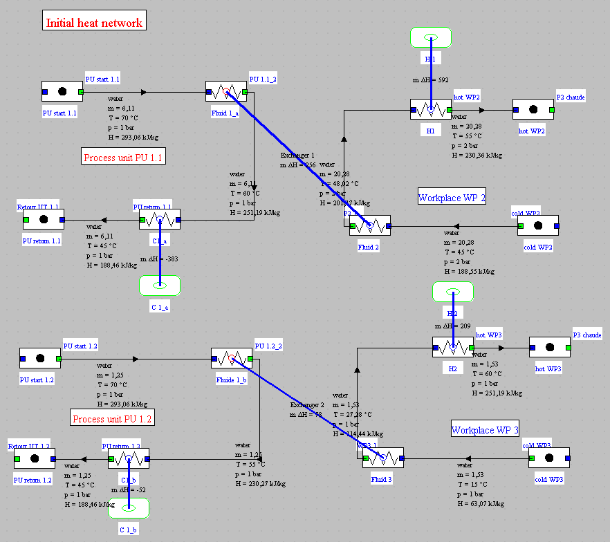
Let's look at the heat exchangers.
The effectiveness epsilon of exchanger 1 is equal to 0.4, and that of exchanger 2 is equal to 0.273.
All are therefore quite small.
Let's see how we can improve them.
For exchanger 1 we will set a pinch equal to 8 °C, which is quite classic for a water-water exchanger.
For the exchanger 2 it can be noted that it is far from using all the thermal power available in process unit 2.
It is therefore possible to set it so that it completely exhausts the fluid 1_b.
With this setting, the screen becomes the following.

The thermal power to be brought drops to 570 kW, a reduction of 29%, and that of cold utilities to 204 kW, a reduction of 53%.
Model retained for optimization by the pinch method
As we know, the application of the pinch method consists in carrying out the analysis of availability and needs from the four fluids involved in the problem.
We build for this the composite curves corresponding to these fluids, which makes it possible to determine where the pinch of the problem is located.
The model does not need to represent the entire existing installation: it is enough for it to show nothing but the fluids involved.
It is therefore much simpler than the one we have just studied, which only had the interest of showing the limits of a "classic" optimization.
Loading the model
The model is loaded by opening the diagram file and an appropriately set project file.
Loading the model
Click on the following link: Open a file in Thermoptim
You can also:
- either open the "Project files/Example catalog" (CtrlE) and select model m7.2 in Chapter 7 model list.
- or directly open the diagram file (opt1RDC_en.dia) using the "File/Open" menu from the diagram editor menu, and the project file (opt1RDC_en.prj) using the "Project files/Load a project " menu from the simulator.
Display the diagram editor window
You see there the diagram of the model, with the four fluids involved, their flow rates, the inlet and outlet temperatures, and the thermal powers exchanged.
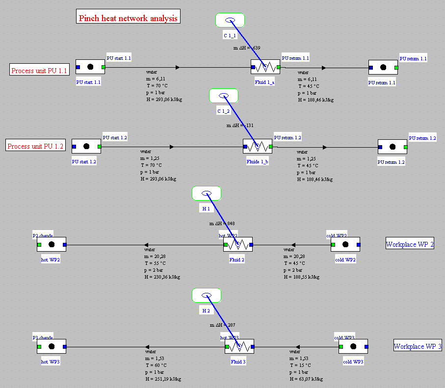
The table below summarizes the data of the optimization problem.
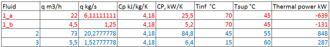
You immediately notice that the first two lines of data differ only in flow and therefore thermal power. The inlet and outlet temperatures and substance Cp are the same.
It would therefore be entirely possible to merge them by summing the flow rates, and to show only three fluids, the first corresponding to this fusion. However, we will not do it here, the fact that the two fluids are analogous poses no difficulty to Thermoptim.
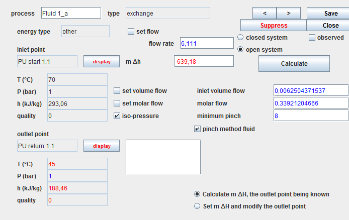
The following figure shows the screen of the process defining fluid 1_a.
For the optimization method, the two main parameters are:
- the "pinch method fluid" option, which must be checked. It means that this process is part of the optimization problem to be treated.
- the value of the minimum pinch, which must be chosen according to
the type of problem posed. As we said before, a value of 8 °C is
suitable for water-water heat exchangers.
In the next step, you will get to know the Thermoptim screen which allows you to use the pinch method.
Presentation of the optimization screen
During this step, you will become familiar with the upper part of the optimization screen.
Optimization screen
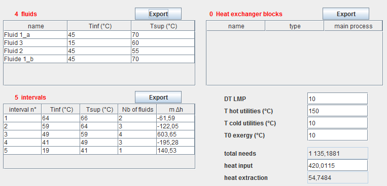
It includes four tables, of which only the first two interest us for this exercise:
- the fluids table contains all the fluids represented by exchange type processes in which the "pinch method fluid" option is selected. These fluids are taken into account by the systemic integration algorithms implemented in Thermoptim.
- the interval table contains the list of intervals constructed by the method.
- the heat exchanger block table contains the exchange blocks which can be defined in order to facilitate stream matching in heat exchangers
- the observed types table shows the points or processes for which
the "observed" option has been checked. These are generally the
elements that are modified during the optimization process, before
performing a recalculation.
In the lower right part of the screen appear several fields, five of which are editable:
- DT LMP is the minimum pinch value used for plotting the locus of minimum pinches. By default it is set to 11 K;
- T hot utilities is the temperature used to plot the hot utility target (heat input requirements). By default it is set to 1,000 K;
- T cold utilities is the temperature used to plot the cold utility target (heat extraction requirements). By default it is set to 300 K;
- T0exergy is the value used for environment temperature reference in exergy calculations. By default it is initialized to the value set in Thermoptim global settings. If it is changed in the optimization screen, this does not affect other exergy calculations performed by the simulator;
- total needs represents the sum of all the enthalpies of the cold streams;
- heat input is the value of the additional heat which may have to be provided to the hot streams if the total needs exceed the heat available when pinches are taken into account. This value is also often referred to as the "energy target";
- heat extraction represents the value of the heat which must be extracted from the system by cold utilities. It should be noted that the existence of pinches explains that, as shown above, there may be at the same time a need for a heat input (at high temperature) and for a heat extraction (at low temperature).
Use of optimization tools
All the optimization-specific functions are accessible from the optimization window.
They work in close coordination with the simulator, so that you may easily modify the settings of the systems studied.
Loading the optimization screen
You access the optimization screen, by typing Ctrl M or by selecting the "Optimization Tools" line from the "Special" menu of the simulator screen.
If you can't do it, click this button
This screen has two menus, as you can see for yourself, the "Optimization method" menu and the "Charts" menu.
Menu "Optimization method"
- target minimization corresponds to the shifted temperature PTA;
- Composite curves CCs, GCC builds up the composite curves;
- Update the problem updates the optimization elements from the process table;
- Update and minimize target combines the third and first items;
- Export the intervals creates a text file named "interv.txt" in subdirectory "pinch" containing all the information on intervals;
- Export the heat exchanger blocks creates a text file named " HXblock.txt" in subdirectory "pinch" containing all the information on the heat exchanger blocks, as well as preliminary computations of the exchanger characteristics (effectiveness, NTU, LMTD, UA value);
- Export the pinch method fluids creates a text file in subdirectory "pinch" containing all the information on the problem data;
Menu "Charts"
- Plot the Carnot Factor curves plots the exergy composite curves;
- Plot the mixed HX-TI Curves plots the composite curves obtained when part of the heat exchanger network is set;
- Plot the CFDC plots only the Carnot Factor Difference Curve;
- Plot composite curves plots all these curves.
Refer to volume 1 of the Thermoptim reference manual for detailed information on all of these concepts.
In practice, however, only two menu lines will be useful:
- Update and minimize target, so that Thermoptim establishes the interval table and calculates the needs for hot and cold utilities
- Plot composite curves to draw these curves
Table of intervals and requirements for hot and cold utilities
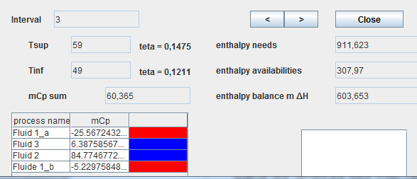
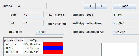
You can examine the content of the intervals by double-clicking on the rows of the table located in the center left of the window.
In the interval windows, hot fluids appear in red, cold fluids in blue.
The upper (Tsup) and lower (Tinf) temperature limits are indicated, as well as the enthalpy needs and availabilities and the net enthalpy balance, which is positive if the heat requirements are higher than the availabilities, and negative if not.
The small arrows at the top right allow you to scroll through the different intervals.
Construction of the interval table
It is now possible to build the interval table from the values on these screens.
For this, report the values of the upper and lower temperatures of each interval in a spreadsheet, as well as the value of its net enthalpy balance.
You fill a table of the type below, the last column being obtained by subtracting the values of the enthalpy balance from the intervals already considered.
This table shows that the maximum enthalpy deficit is equal to 420 kW, in the absence of the boiler, and that it takes place at the level of interval 3.
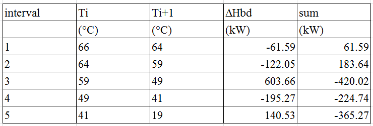
This is where the pinch of the system is located. Given the value of the minimum pinch retained (8 °C), this corresponds to 53 °C for the donor fluids (hot), and to 45 °C for the receiver fluids (cold). The deficit must be compensated by an addition of hot utilities equal to 420 kW.
If we modify the table by bringing this power at high temperature, we obtain the following figure where the pinch corresponds to the interval whose total cumulative balance is equal to 0.
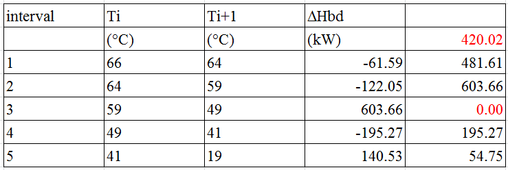
Recall that this table is related to the temperatures shifted by half the value of the minimum pinch which are those used by the pinch method to find the optimum.
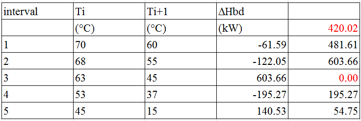
To obtain the table relating to actual temperatures, simply subtract 8/2 = 4 °C from cold fluids, and add 4 °C to hot fluids, as shown in the following figure.
Plotting composite curves
The composite curves are drawn by activating the Plot composite curves line in the Charts menu.
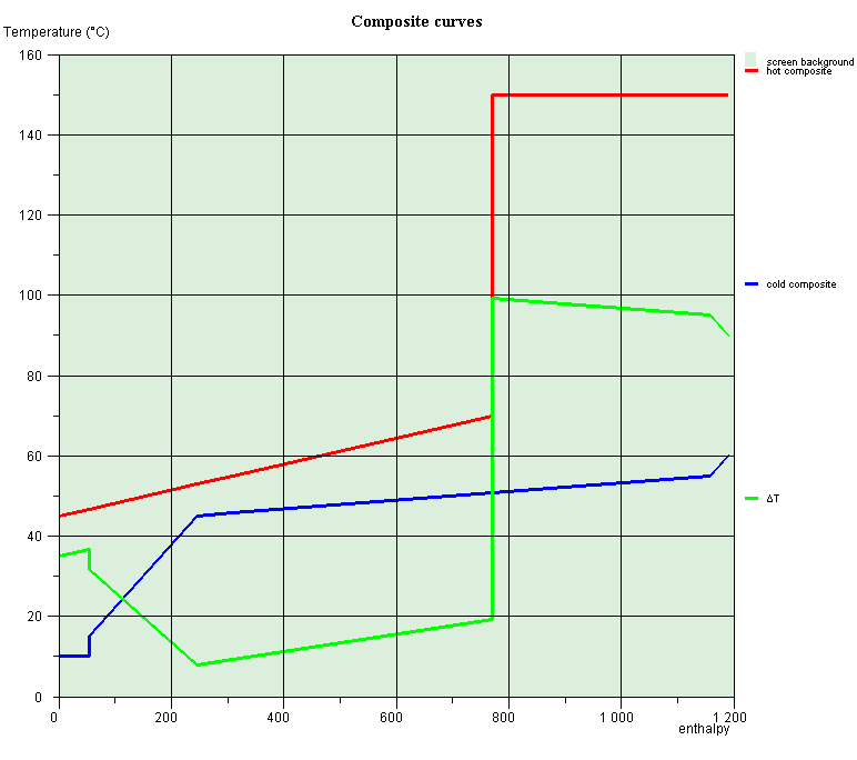
The red curve corresponds to the hot composite, the blue curve to the cold composite, and the green is the difference between the two.
The pinch appears clearly on the abscissa 247 (kW), for a temperature of 45 °C at the level of the cold fluid, and 53 °C for the hot fluid.
On composite curves, the pinch separates two areas:
- the upper zone where the heat requirements of "cold" fluids are greater than the enthalpy available in "hot" fluids, and additional heating is necessary. This zone, deficient in heat, behaves as a heat sink, and is called endothermic zone.
- the lower zone, where the situation is dual from the previous one:
"cold" fluids (needs) are unable to absorb all the heat available in
"hot" fluids (availability), a surplus having to be evacuated by a
complementary cooling fluid. This zone, excess heat, generally
behaves like a heat source, and is called exothermic zone;
The requirements for hot and cold utilities can be read on the abscissa of the graph.
The two values displayed in the optimization screen are found, namely 420 kW and 54.7 kW respectively.
The needs for hot utilities are reduced by 47.6%, but those for cold utilities have decreased by 87.4%, going from 436 kW to 54.7 kW.
If we now compare them to the results of "classic" optimization, the need for hot utilities is reduced by 26.3% and those of cold utilities by 73%, which is considerable.
These results illustrate the capacity of the pinch method.
Construction of the optimized heat exchanger network
It is now possible to study the optimized heat exchanger network.
The procedure is as follows:
- separate the study of endo and exothermic zones;
- begin the study at the pinch, and deviate gradually, in order to deal with the most constrained problem first;
- only import energy into the endothermic zone, export only from the exothermic zone;
- Maximize the load of the exchangers (in order to minimize their
number).
This procedure can be quite complex in some cases, but, for this example, it does not pose any particular problem.
Analysis of intervals located at the pinch
We must begin by examining the intervals located at the pinch.
It is clear that, below the pinch, the only cold fluid which appears is fluid 3.
It must therefore be paired with the hot fluids available, and the charge of this exchanger should be maximized.
Construction of the exothermic zone exchanger
As there is only one cold fluid and the two hot fluids are the same except for the flow rate, we will mix them so that they constitute only one fluid, which we will call "Fluid 1", which we subdivide into two exchange processes in series, "Fluid 1_1" and "Fluid 1_2".
The intermediate point between these two processs (mix 2), which is located at the pinch, is therefore at 53 °C (hot fluid).
Downstream of the latter, we add a new process "C1" to represent the cold utilities for cooling Fluid 1 to 45 °C.
In the same way, we add, downstream of the two processes "Fluid 2" and "Fluid 3", two new processes "H1" and "H2" to represent the hot utilities.
For these three processes representing the hot and cold utilities, the option "pinch method fluid" must be unchecked.
The point between Fluid 3 and H2 (WP3_1), also at the pinch, is therefore at 45 °C (cold fluid).
Finally, Fluid 1_2 and Fluid 3 can be coupled by an exchanger, called E2.
We arrive at a diagram of this type.
The setting of the E2 exchanger is as follows.
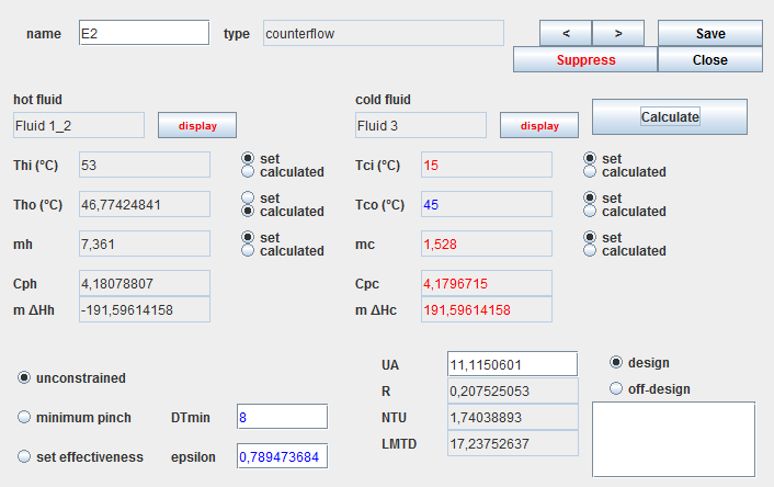
The inlet and outlet temperatures of fluid 3 are known, as well as its flow rate.
The inlet temperature of fluid 1 is known, as well as its flow
Five constraints being set, the exchanger is calculable, and the outlet temperature of fluid 1 can be determined.
The effectiveness of this exchanger is 0.79.
Construction of the endothermic zone exchanger
To finalize the network, simply couple Fluid 1_1 and Fluid 2 processes by an exchanger E1 whose setting is as follows.
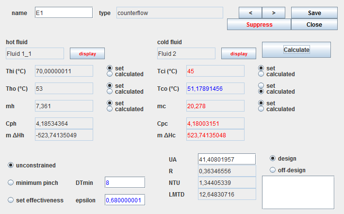
The inlet and outlet temperatures of fluid 1_1 are known, as well as its flow rate.
The inlet temperature of fluid 2 is known, as well as its flow rate.
Five constraints being set, the exchanger is calculable, and the outlet temperature of fluid 2 can be determined.
The effectiveness of this exchanger is equal to 0.68.
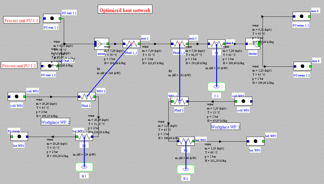
Synoptic view of the optimized installation
We arrive at a diagram of this type.
Loading the model
Click on the following link: Open a file in Thermoptim
You can also:
- either open the "Project files/Example catalog" (CtrlE) and select model m7.3 in Chapter 7 model list.
- or directly open the diagram file (opt1RDC_Ech_en.dia) using the "File/Open" menu from the diagram editor menu, and the project file (opt1RDC_Ech_en.prj) using the "Project files/Load a project " menu from the simulator.
As you can easily check, the sum of the power inputs required for hot utilities is 420 kW, and the cooling power for fluid 1 is 55 kW.
This heat exchanger network therefore corresponds well to the optimum highlighted by the pinch method.
Conclusion
This exploration allowed you to discover how the pinch method can be applied to optimize a heat network.
You will find more detailed information on this subject in the following two pages of the Thermoptim-UNIT portal:
Heat integration or pinch method
Presentation of the Thermoptim optimization method
If you wish to study this heating network in greater depth, another guided exploration (DTNN-3) will explain to you:- how to size the two exchangers E1 and E2 that we have just designed,
- and how to compare the exergy balances of the initial installation and the optimized one.
Activate the menu item Update and minimize target.
Thermoptim establishes the interval table and calculates the needs for hot and cold utilities.
A message informs you that an additional 420 kW is required and asks you if you want to save this value.
Answer "OK"
Remember that the total power to be supplied by hot utilities in the existing installation is 801 kW.
The application of the optimization method shows that there is a network of exchangers allowing to save 47.6% of heat input by hot utilities!