Psychrometric chart user's manual
Table of contents
© R. GICQUEL 1998 - 2022. All rights reserved. This document may not be reproduced in whole or in part without the author’s express written permission, except for the personal licensee’s use and solely in accordance with the contractual terms indicated in the software license agreement.
Information in this document is subject to change without notice and does not represent a commitment on the part of the author.
Overall presentation
The THERMOPTIM ® series (www.thermoptim.org) is a set of software tools dedicated to the learning and better understanding of applied thermodynamics. It is comprised of easy to use interactive charts: ideal gases, vapors mixtures of an ideal gas and of water vapor (psychrometrics), and a modeling software package including four closely interconnected working environments : a diagram editor (synoptic screen), a simulator, the interactive charts, and an optimization tool.
The interactive charts have been developed with a view to replace classical paper thermodynamic charts. Indeed, whatever care is taken by editors in the choice of color sets for distinguishing the various curves shown on the classical charts, it is always difficult to read them, and interpolation may lead to significant errors. New THERMOPTIM charts allow one, by a simple mouse click, to display all relevant thermodynamic properties of the fluid, thus providing better accuracy. Their main asset is to be very easy to use: the thermodynamic properties are immediately displayed on the screen, a user-friendly point editor allows the user to refine his/her cycle analysis and to export the values in spreadsheets or text editors.
THERMOPTIM is applied thermodynamics software whose objective is to allow one to easily calculate complex thermodynamic cycles without making very simplistic hypotheses or without being involved in tedious calculations. Initially it has been developed to help solve problems encountered in teaching applied thermodynamics. Its present functionalities make it possible to use it for also solving much more complicated problems such as industrial schematic design (for instance it has been used for the system integration of advanced electricity generation production plants involving several hundreds of components).
In this manual, we shall present the psychrometric charts, successively showing how to :
- use the chart to display a point and recalculate it
- customize the working environnement (gas selection, calculation settings, choice of the line width and color, layout of the axes…)
- work with point selections (named cycles), saving and loading them
- edit a compound gas
- print a chart and exit the application
Thermodynamic properties of substances
The software includes a data base with the thermophysical properties of the substances considered. It makes use of three kinds of substances: pure ideal gases, compound ideal gases and water considered as a condensable vapor. Perfect gases are ideal gases whose specific heat is independant of the temperature (let us recall that the equation of state of an ideal or perfect gas is Pv = rT).
The substance can be pure, in which case its properties are predefined in the software, or it can be compound. In this case (that is possible only for a gas), the user has to define the composition from the other gases present in the database, by indicating for each of them, its name and its molar or mass fraction. Properties of the composed substance are then determined from those of its constituents. Two sets of compound gases exist: protected and non protected gases. This difference has been introduced in order to avoid that some gases whose composition dos not vary, such as air, be inadvertantly modified by a user. Only non protected gases may be modified and saved.
The accuracy of the calculations is excellent for ideal gases (error on the specific heat lower than 0.5 % as compared with Janaf tables), and for water (comparative tests with ASME steam tables give, for compressions and expansions, relative errors with enthalpies lower than 0.02 % in the vapor and liquid-vapor equilibrium, and lower than 0.5 % for the compressions in the liquid state).
Detailed information on the equations used can be found in the following reference:
Energy Systems, A New Approach to Engineering Thermodynamics, 2011
Energy Systems, A New Approach to Engineering Thermodynamics, 2nd Edition, 2021
Internationalisation, number formatting
The interactive charts exist in several languages (english, french, spanish, portuguese, catalan). They are configured in the language corresponding to the inth.zip file located in the installation directory.
Numbers are automatically formatted in accordance with the language selected in the computer system. For instance, in english, the decimal separator is the dot, and the thousand one the comma ; in french the decimal separator is the comma, and the thousand one the space.
If you enter an ill-formated number, it is truncated at the level of the first non numerical character.
Chart use, display and recalculation of a point
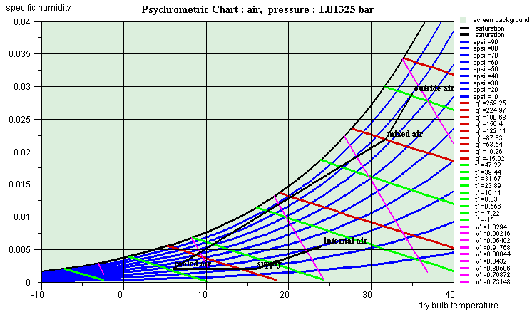
Using the interactive charts is quite simple: position the crosshair cursor at the point whose thermodynamic properties you wish to get, and click so that they may be displayed on the screen. For psychrometric charts these properties are: absolute humidity (dimensionless ratio of the water mass to the dry gas mass unit), relative humidity (dimensionless), water vapor partial pressure (Pa), dry bulb temperature (°C), wet bulb temperature (°C), adiabatic temperature (°C), specific enthalpy (kJ/kg) and volume (m3/kg) (relative to the dry gas mass unit).
As the cursor positionning accuracy is a function of the screen resolution and is generally not very high, it is possible to make more precise calculations either by moving a target with the keyboard arrows, or by creating and editing points (named cycle points as a set of points usually represents a thermodynamical cycle).
Using keyboard arrows
It is possible to refine the positionning of the cursor with the keyboard arrows. To do that, click close to the point whose properties you wish to get. The values are displayed in blue above the chart. If you press one of the keyboard arrows, a red target appears and is moved in one of the four cardinal directions by an increment equal to 1/1000 of the horizontal or vertical scale depending on the arrow key used. The point properties are recalculated, so that you can gradually get closer to the desired point. By changing the chart scale as indicated in the section entitled "Changing the axes layout", you can change the displacement sensitivity.
As soon as the red target appears, the mouse click is disabled, and the target can only be moved by the keyboard arrows. To take control again on the cursor, you can either :
- press the "Escape" key. The red target disappears and is displayed again only when you press one of the arrows, close to the location you last clicked the mouse. If you have not clicked since it disappeared, it appears where it previously was.
- double-click, which creates a point (see below) positionned on the target.
Point creation
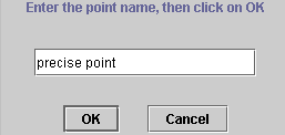
To create a point, double-click at the requested location. A dialog frame asks you to enter a name to identify the point.
Once the point is named it is displayed on the screen in the form of a little cross and its label.
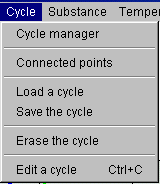
You can open an editor which allows you to modify the point and recalculate it. To do that, select the menu item "Edit a cycle" of menu "Cycle" or type Control C:
The cycle editor is then displayed. In its upper zone there are text fields which allow you to add comments on the cycle if you wish to do so, in particular for saving the cycle. The title is used for identifying the cycle in the cycle manager (see below). If you simply wish to recalculate a point, this is not necessary. In the lower part of the screen is a table comprising in columns the name of the point and its thermodynamic properties, and in lines each point entered (only one at this stage).
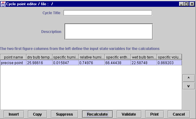
All the possibilities offered by the cycle point editor will be presented in detail later. For the time being, we will just show how to recalculate a point.
The point table has a particular feature: you can change the column order by clicking and dragging one of them by its label. For instance, if you click on the label "dry bulb temperature" and that, keeping the mouse pressed, you move it on the right, the absolute humidity column automatically is shifted to the second location.
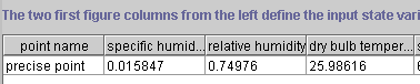
If you keep on moving in the right direction, the relative humidity column is shifted in turn, and so on. After two moves, you get the following result:
THERMOPTIM interactive charts make use of this editor property to specify the input variables used when a point is calculated: the two first figure columns from the left are considered by the software as designing the known state variables from which the other thermodynamic properties are calculated.
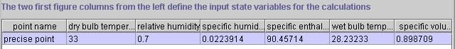
Suppose that you wish to calculate a point with a relative humidity equal to 70 % and a dry temperature of 33 °C. Enter these values in the corresponding cells, making sure to indicate that the cell editing is finished by pressing enter or clicking in another cell. Click then on button "Recalculate" located in the lower right part of the editor. The point is recalculated and the values displayed :
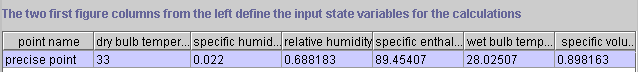
If you wish the point with a dry temperature of 33 °C and an absolute humidity of 0.022 kg/kg, move the absolute humidity column in second or third position, enter this value, then click on button "Recalculate". You get the following result (here the editor window has been resized and the width of some columns modified):
As you can see, calculating a point with accuracy is very easy.
All variable couples comprising the dry temperature or the absolute humidity can be calculated.
Once the point is recalculated as you wish, the modifications made in the editor can be transferred on the chart by clicking on button "Validate". Automatically, the editor table points are then repositionned on the screen.
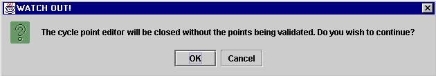
Once you are back in the main chart window, you can enter additional points. If you want to display them in the cycle points editor, you must select again menu item "Edit a cycle" of menu "Cycle". If the editor was previously opened, a message informs you that the points will not be validated if you continue.
The reason for this is that the software cannot guess which values are the right ones: those from the chart or those from the editor. If you do not want to validate the points previously modified, click on "OK". Otherwise cancel, and then go into the editor, validate the old points, and iterate.
Customizing the working environnement
The working environnement of THERMOPTIM interactive charts can be customized in several ways so that you can adapt it to your own taste. When you first run the software, default values are used. Subsequently, your modifications are automatically saved in various configuration files, so that your selections are kept between two sessions.
Gas selection
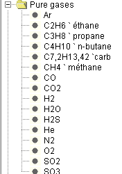
The software contains about fifteen pure gases which can be used to constitute as many compound gases as you wish.
The compound gases can either be defined in an editor, or chosen from among the list of existing gases.
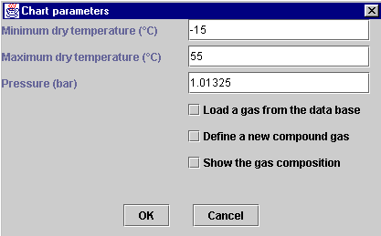
In either case, to modify the selected gas, you select the menu item "parameters" of menu "Chart", and the following window is displayed:
Choosing a gas in the data base
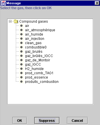
If you select the checkbox "Load a gas from the data base", the list of available pure and compound gases is displayed.
Select the gas whose psychrometric chart you wish to build (here "gas_brulés"), then click on "OK".
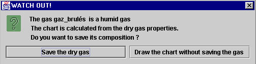
In this example, it is a combustion flue gas, which contains water. The gas is therefore a moist gas, whereas the psychrometric chart is built from the dry gas. The dry gas composition is automatically calculated by the software, and a message proposes either to save it, or to directly plot the chart.
If you wish to save the dry gas, you have to name it. Otherwise, Thermoptim creates an temporary dry gas which is not listed among the compound gases.
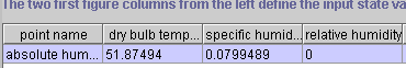
In either case, the chart is built for the selected gas, from its dry composition. In addition, a new point is created to save the absolute humidity of the moist gas, the dry temperature being arbitrarily chosen close to the saturation curve. It is indeed interesting to save the absolute humidity value if you wish to plot on the chart points with exactly the same humidity as the initial moist gas (for a (w,t) chart, all the points corresponding to this humid gas are located on the horizontal line on the right of the saturation curve containing th point created).
This point can be displayed in the cycle point editor, and thus recalculated as you may wish. You just have to enter for instance the dry temperature.
Definition of a new compound gas
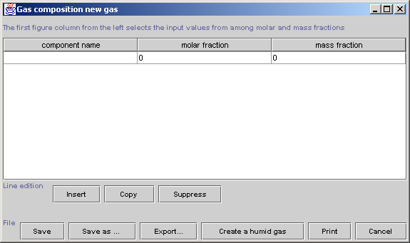
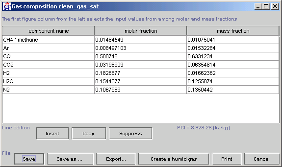
If you select checkbox "Define a new compound gas", the software asks you first to name it, and then opens the gas composition editor, which is similar to the cycle point editor we saw previously, but also presents some differences.
There are only three columns in this editor: the first one contains the pure gases available in the data base, and the two other ones are used to enter the molar and mass fractions. You Thermoptim considers that the first column of numbers on the left contains the data to be taken into account, the others being calculated from those (you can move a column by clicking on its headband and dragging it laterally). However, if you choose to enter the mass fractions, it is necessary that the values of the molar fractions are set to 0. Obviously, the sum of the mole or mass fractions must be equal to 1.
To define a compound gas, choose from along the list of pure gases in the constituent column (which is displayed when you click in the corresponding cell), then enter its molar or mass fraction. Insert then a new line by clicking on the button "Insert", and define similarly a second constituent, a third one, etc.
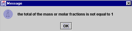
When you are done with entering constituent lines, validate by clicking on "Save". The software checks that the sum of the molar or mass fractions is equal to 1. If this is not true, the gas cannot be saved and a message informs you.
You can however ask the software to complement to 1 the sum of the molar or mass fractions, by calculating that of one of the components that you leave undetermined, by entering no value in the corresponding field. Only the first undetermined value is taken into account, the other ones being set to 0. Furthermore, molar or mass fractions must obviously be positive.

If the gas composition is consistent, the gas is saved and its molar and mass fractions recalculated, as in the following example. Then the chart is built and displayed.
The gas editor is equipped with other buttons which will be presented later.
Selection of the chart type
The substance properties can be displayed in several coordinate systems used by thermodynamicians.
For mixtures of an ideal gas and water vapor, the following charts are available:
- (t,w) psychrometric chart, with dry bulb temperature in abscissa and specific humidity in ordinate ;
- (w,q') Mollier chart, with specific humidity in abscissa and specific enthalpy in ordinate.
To select one of the types, click on the corresponding menu item. The screen is immediately updated.
Choosing the line width
By default, the curves are plotted in bold line.You can reduce the line width by clicking on the menu item "narrow line" of the menu "Chart". It is then labelled "bold line". If you select it subsequently the lines are again plotted in bold lines.
Modifying drawing and screen background colors
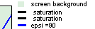
The whole set of colors used for plotting curves and for the screen background can be customized. To modify a color, double-click on one of the small rectangles where it appears in the legend on the right of the screen:
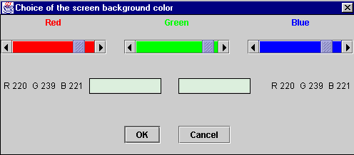
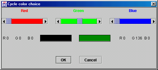
The following color editor is displayed (this example retates to the screen background color).
Three cursors corresponding to the red, green and blue components of the color allow you to customize the color. In the rectangle located center left, the original color is displayed, whereas the new one is shown in the right one, reflecting the cursor moves. When you have made your selection, click on "OK". The color is saved.
Changing the axes layout
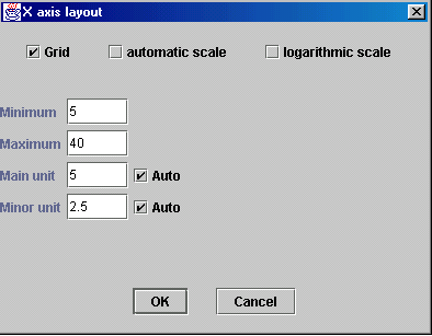
The abscissa and ordinate axes layout can be modified by selecting the menu item "X Axis" ou "Y Axis" of menu "Chart". This window is then displayed.
If you select the checkbox "Grid", vertical lines for the abscissa axis and horizontal lines for the ordinate axis are plotted on the chart, at the main unit tick.
If you select the checkbox "automatic scale", the software searches a scale covering the whole range of values. The scale is logarithmic if you select the corresponding checkbox, linear otherwise.
When the "automatic scale" checkbox is not selected, you can enter the minimum and maximum values that you wish. The values of the main and minor units can be either automatically calculated, either entered by you, depending whether the corresponding "Auto" checkbox is selected or not. If the unit values are not consistent with those of the minimum and maximum or between themselves, a beep warns you.
Watch out: if the "automatic scale" checkbox is selected, your values will be replaced by those that the software will calculate.
When you are done with your modifications, click on "OK" to save the new layout, or on "Cancel" to go back to the previous values.
Other chart parameters
By selecting the menu item "parameters" of menu "Chart", you may modify either the pressure used for building the psychrometric chart, or the bounds of the calculation interval for dry bulb temperatures. As a matter of fact, as the chart is continuously recalculated, either ten iso-values per property are automatically plotted as a function of the working interval defined by the user, in order to obtain a good readability, or the iso-values plotted are those defined by the user (see section "Selection of the isovalues").
The minimum and maximum values of the calculation interval for dry bulb temperatures are in addition used by the cycle point editor, to get the possible bounds of the various thermodynamical properties used as data. If you enter a value which is out of limits, the calculation is impossible and a message warns you that you attempt to calculate a value which cannot be reached. The solution is therefore either to modify the requested value, or to change the temperature interval.
Lastly you can edit the composition of the gas for which the chart is built. To do this select the checkbox "Show the gas composition" of the parameter window. The gas composition editor is then displayed. You can modify it if you wish. To save these modifications, click either "Save", which modifies accordingly the composition of the selected gas, or "Save as", which allows you to save your modifications by creating a new gas.
Cycle handling
You have previously learnt how to create and modify points. In next pages, we shall refer to a set of points as a cycle.
Point creation from the cycle editor
In addition to the recalculation and validation functions discussed previously, the cycle editor is equipped with five other buttons : "Insert", "Copy" and "Suppress", which allow you to add, copy or suppress one table line, and "Print" and "Cancel" which allow you to print the table or to close the frame. Furthermore, on the right of the frame appear two small arrows which can be used to move a line to the next above or below position.
To add a new point, select one line, then click on "Insert". The software inserts a new line just above the previous one, all the values being set to zero. Name this new point, choose two input variables, move the corresponding columns on the left and enter their values, then click on "Recalculate" to get all the point thermodynamical properties.
Once the new line is inserted, you can also copy another line and paste it. To do that, select the line corresponding to the point that you wish to copy, and click on "Copy". The button label is modified and becomes "Paste". Select the destination line, and click on "Paste". The values are copied.
To suppress a line, select it then click on "Suppress". Once the points are created as you wish, click on "Validate" to have them transferred on the chart and displayed. To print the table, click on "Print" and select the paper format from the printer dialogs, then confirm the printing.
Connecting points
When the points are displayed on the chart, they are disconnected by default. It is possible to connect them by a broken line by selecting the menu item "Connected points" of menu "Cycle". This way of doing is widely used for representing a thermodynamical cycle. In the following example is shown an air conditioning cycle:
The software connects the points in the same order as they appear in the editor, starting from the first line. If this order is not the right one, you may have to sort the points in the cycle editor.
To do that you can move the points using the arrows which appear in the right of the editor:
- select a line that you wish to move
- click on the up or down arrow to move the point to the previous or next line position
- when you have rearranged all points, end up by clicking on "Validate". The cycle is then displayed on the chart in the right order.
Cycle manager
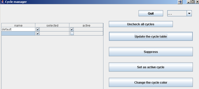
A new menu line named "Cycle manager" has been added in menu "Cycle". If you select it you open this frame. If you click on "Update the cycle table", all cycles already loaded are displayed. Here, two cycles are loaded: the default one which is active, and a second one which has been loaded from a file.
The title defined in the cycle point editor is displayed as the cycle name.
You select the active cycle by choosing its line and clicking on "Set as active cycle". The active cycle has the following properties:
- it is connected to the simulator (when the charts used are connected to Thermoptim) ;
- it is the one on which the "Cycle" menu lines operate, i.e. it can be erased, saved, its points can be edited in the cycle point editor...
If you double-click on a line, you change the column "selected" status: if it is checked, the cycle is plotted on the chart, otherwise not. You can deselect all cycles by clicking on "Uncheck all cycles". You can suppress a cycle in the list by selecting its line and clicking on "Suppress". Its plot is also suppressed from the chart.
In the upper right of the screen is a multiple choice list that lets you choose the kind of plot of the selected cycle: solid line, dotted or dashed.
Changing the cycle color
Until version 1.3, all cycles were plotted in black. It is now possible to select any color in the same way as you do it for the chart curves. To change a cycle color, select its line and click on "Change the cycle color". A frame allowing you to choose its color is displayed. If you want to save the new color, set the cycle as the active one and save it. Suppressing the active cycle is equivalent to erasing it from the chart menu. You generate a new active cycle either by setting another cycle as the active one, or by interactively creating points in the chart, opening the cycle point editor and validating.
Superposition of several cycles on a chart
To plot several cycles on a chart, just load them together and set them as selected in the cycle manager screen.
Erasing a cycle
It is possible to erase a cycle displayed on the screen: to do that, select menu item "Erase the cycle" of menu "Cycle". This operation suppresses the corresponding point values, which cannot be displayed again if the cycle has not been saved. If you just wish to hide a cycle from the screen, unselect it in the cycle manager frame by double-clicking on its line.
Saving a cycle
Once a set of points has been entered, and possibly recalculated and validated, it can be saved as an ASCII text file, in order to be subsequently processed either by the software, or by a spreadsheet or a text editor. To do that, select the menu item "Save the cycle" of menu "Cycle". A dialog window allowing you to name the file is shown. Name it and click on "Save" to save the cycle.
Loading a cycle
You can import in the software, either for displaying it or to process it, a cycle which has been saved previously, or created in another working environment. To do that you just have to configure a data file structured as below.
In this example the file has been created by the software, but any file structured similarly can be read and processed. The line separator is the 'Enter' character, and the column separator the tabulation.
The two first lines are not taken into account (but they must exist). The third one provides various information: here the cycle is in colour and has been saved in a universal way (i.e. with the english format).
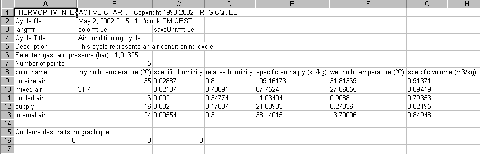
The fourth and fifth lines give in second column the cycle title and a comment describing it. If the first column cells are empty, these informations are not read.
The sixth line first column must include a text in which appears the name of the substance used (in order to warn the user if the substance selected for the chart is not the same as that for which the cycle has been calculated). The pressure is indicated as a reminder but it is not read.
The seventh line first column must be a non-empty text, and the second one the number of points.
The eighth line is not taken into account (but it must exist)
The following lines give the name and the values of the points, in the order given in the above example: name, dry bulb temperature, specific humidity, relative humidity, specific enthalpy, wet bulb temperature, specific volume.
The two last lines define the cycle color with a RGB coding.
Any file structured similarly can be read by the software.
To import a cycle file, select the menu item "Load a cycle" of menu "Cycle". A dialog window allows you to select the file.
If some points have already been created, or if another cycle has been loaded, a message warns you. If you cancel, existing points are not modified, and the cycle is not loaded. If you continue the loading, the existing points are suppressed and replaced by the new ones.
Compound gas editor
The software includes a compound gas editor which we rapidly presented when introducing the definition of a new gas. In this section, we shall give details on the different possibilities of this editor, as well as on the functions of menu "Gas Editor". We have explained previously how a compound gas can be defined or modified. We shall present here the available functions for saving, suppressing, exporting or importing compound gases in the software data base.
You can open several compound gas editors at the same time, and the gases which they display are not necessarily the one which corresponds to the psychrometric chart.
The three first lines of menu "Gas Editor" operate in the same way as the actions available in the parameter screen.
Loading a gas from the data base
The first line opens the pure and compound gas selection window, in which you select a new gas whose chart is then plotted.
Displaying the gas composition
The second line allows you to display the composition of the selected gas.
Creation of a new gas
The third line allows you to create a new gas.
Editing a gas, functions of the gas editor
To edit a gas, select the menu item "Edit a gas…" of menu "Gas Editor".
A screen similar to that which allowed to choose the gas for the chart is displayed. There are two differences:
- only available compound gases are shown, as editing a pure gas does not make sense
- a button "Suppress" allows you to suppress from the compound gas list those which you do not need any more. Select them turn in turn, then click on the button. A confirmation message allows you to cancel in case of error.
If you select a gas and click on "OK", its composition appears in the editor.
You can modify the gas composition, by choosing the constituent names in the list of pure gases which is shown when you click in the first comlumn cells, and entering either the molar or the mass fractions. Once it is defined, the compound gas can be:
- saved, by clicking on "Save". The software checks that the sum of the fractions is equal to 1, and then saves the gas. If the sum differs from 1, nothing is done, except if you have left undetermined a fraction value (see above).
- renamed, by clicking on "Save as…". The test on the sum of the fractions is made, and the gas saved with the new name that you have entered.
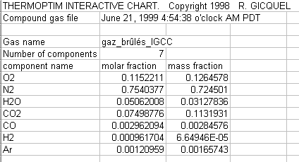
- exported, by clicking on "Export…". The gas composition is then copied in a text file that you name, and that you can open with a spreadsheet or a text editor. For instance, the previous gas can be exported with the following format.
- you can also create, from the gas displayed in the editor, a moist gas of a given absolute humidity. To do that, click on "Create a humid gas". The software asks you to enter the gas name and the absolute humidity requested, and then creates a new compound gas, whose dry gas is the same as that of the gas displayed in the editor, and with the given absolute humidity. This gas is added to the list of compound gases of the data base. You get access to it by the previous screens.
- lastly, if you cancel, the compound gas editor is closed.
Importing a gas
As you can export a gas in the form of a text file, it is possible to import one by selecting the menu item "Import a gas" of menu "Gas Editor". The file format must be the same as that which is used for export files.
The data which are read are the following : the second cell of the fourth and fifth lines, which give the name of the gas and the number of constituents, and the three first cells of lines seven and next, depending on the number of constituents, which give their names and molar and mass fractions.
The first cells of the fourth and fifth lines are not read, but must not be blank. Lines 1 to 3 and 6 must also exist and not be blank.
Printing a chart, end of session
Printing a chart
Printing a chart can be done either from the menu item "Print" of menu "File", or by the keyboard accelerator Control P. A printer selection screen is then displayed.
End of session
To quit the application, you can do it either from the menu item "Quit" of menu "File", either using the keyboard accelerator Control Q. A confirmation screen is displayed. The environnement parameters are automatically saved.
Selection of isovalues for the psychrometric charts
Psychrometric charts can be used for a large variety of dry gases, in any temperature intervals and for the pressure defined by the user.
In order to get a screen background display fitted to a given parameter setting, isovalues to be plotted for relative humidity, specific enthalpy, wet bulb temperature and specific volume have to be recalculated as a function of the choices made by the user. This is what is done by default in the interactive psychrometric charts. This solution allows for the automatic update of the chart screen background, but some users prefer to select by themselves the isovalues to be displayed, in particular to be able to easily interpolate between the curves once they are printed.
In order to meet this requirement the software has been modified and now handles two definition modes for the isovalues: the automatic initial mode, and a new one in which they are set. The isovalues set are read in a specific text file named "isopsy.txt" located in sub-directory "data" of the installation directory.
This file has the followingstructure:
Definition file of isovaleurues for a psychrometric chart
epsilon nepsi=9
0.1 0.2 0.3 0.4 0.5 0.6 0.7 0.8 0.9
qprime nqprime=13
100 200 300 400 500 600 700 800 900 1000 1200 1400 1600
tprime ntprime=11
30 35 40 45 50 55 60 65 70 72 74
vprime nvprime=5
0.8 1.6 1.8 2 2.2 2.5
After the label of each isovalue type, separated by a tab, is given the number of values to be plotted, for example nepsi=9. The integer located after the equality gives the number of values to be read in the following line. The rules are that this integer be lower than or equal to the number of values in the following line, and that the total of the isovalue numbers be lower than or equal to 58 (instead of 36 in the automatic mode).
This file can be built either thanks to a text editor or a spreadsheet, or directly from the software, thanks to a specific interface.
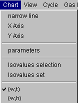
Two new lines have been added to menu "Chart" :
"Isovalues selection" opens a frame with tabs showing the list of the current isovalues, and allowing one to modify, adding or deleting them.
"Isovalues set" changes the operating mode from automatic calculation of isovalues to that in which they are set by the user.
Isovalues selection
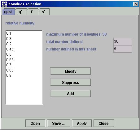
The tab frame allowing to edit isovalues is shown here.
To modify one you select it then click on button "Modify". The selected value is displayed in a window wher you can enter the value you wish to set. Act similarly to delete one.
To add a value, select one, then click on "Add". The new value is inserted before that which was selected, or added in the last position if no value was selected.
It should be noted that relative humidities are expressed algebrically, and not as a percentage.
The maximum isovalue number (58) is displayed, as well as the total number of those which are already defined (here 36), and the number of those which are defined in the current sheet (her 9 for relative humidities).
By clicking on another tab, you change the isovalue type, so that you may set them as you wish.
Once your selection entered, you can define it as the isovalue set to take into account for the current chart by clicking on button "Apply". It is then saved in text file "isopsy.txt" of sub-directory "data" of the installation directory. The previous isovalue set is erased.
Building a library of isovalues files
By clicking on button "Save", you may save the isovalue set you have entered in order to keep it. It is then saved under the name you choose in sub-directory "isoval" " of the installation directory. Subsequently you may open it to load it or modify it (button "Open"). This enables you to build up a library of isovalue sets you can use with different chart parameter settings. You just have to open an existing file and to click on "Apply" to have it replace the previously selected set.
Non-convergence of inversion algorithms
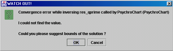
Watch out : if the isovalue set selected is not compatible with the chart parameter settings, the software may be faced with non-convergence problems when it tries to solve equations. Such messages may be shown:
You may either answer "OK" and provide the temperature interval bounds for each calculation, which is tedious, or click on "Cancel", which is faster.
If you want to avoid this unpleasant situation, begin by letting the software automatically calculate an isovalue set consistent with the parameter settings, and choose your own isovalues with values comprised between the limits of the values displayed, or modify your chart's parameter settings (mainly the minimum et maximum temperatures) so that the calculated values more or less correspond to your choices.
Selecting isovalue curve display
Menu "View" allows you to select the isovalue curves which are displayed on the screen.
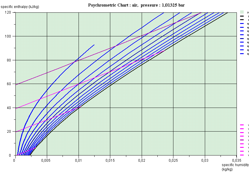
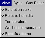
Only those isovalues whose name is checked are plotted. If for instance you check only the saturation curve, relative humidity and wet bulb temperature, the chart looks as follows: