Thermoptim reference manual Volume 4
Table of contents
© R. GICQUEL 1997 - 2022. All Rights Reserved. This document may not be reproduced in part nor in whole without the author’s express written consent, except for the licensee’s personal use and solely in accordance with the contractual terms indicated in the software license agreement.
Information in this document is subject to change without notice and does not represent a commitment on the part of the author.
1 Introduction
In this Volume 4 we present a series of developments that have been made on the one hand to allow completion of the Thermoptim core in order to address much more complex modeling than those presented in the other reference manuals, and on the other hand to automatically derive productive structures, namely in order to obtain precise exergy balances.
1.1 Technological design and off-design operation
Modeling developments allow one to:
- drive Thermoptim calculations taking control on the automatic recalculation engine;
- perform technological design and conduct studies of the behavior of systems operating off-design.
Given the extent of the area corresponding to these problems, we do not claim to provide them with comprehensive answers: we limit our ambition to provide a few relatively simple examples illustrating the potential of drivers and tools dedicated to technological design and off-design operation.
Advanced users willing to solve specific problems will have the task of building their own relevant models. The examples presented should be considered only as templates intended to be refined by users who wish to study the technological design and off-design behavior of systems, and not as well validated models. Our goal is simply to facilitate their efforts by providing them with practical examples on which they can elaborate.
Let us emphasize that this is an extremely interesting though very difficult topic, little addressed so far, probably because of lack of an appropriate tool, but essential if one wants to really understand how real machines behave. This document being a software reference manual, we will not develop thermodynamic analyses. We refer to Part 5 of the book Energy Systems the reader interested in further developments in this regard.
GICQUEL R., Energy Systems: A New Approach to Engineering Thermodynamics, January 2012, CRC Press, ISBN-13: 978-0415685009.
Until 2008, the component models used in Thermoptim were rather simple: the phenomenological models built certainly allowed to study the thermodynamic cycle of the technology under consideration, but not to perform a specific technological design, or simulate performance in off-design operation, the latter two issues being much more complex than the first. To address these issues, we have been led to distinguish two levels in the models (their name was chosen to be as clear as possible, but it is not usual):
- phenomenological models, the only so far implemented in Thermoptim allow accurate calculation of thermodynamic cycles, regardless of the choice of a particular component technology;
- technological design and off-design operation simulation models not only provide the same results as the previous ones, but thanks to the inclusion of additional equations specific to the technologies chosen, allow more precise sizing of the various components and, once the technological design made, enable you to study the behavior of the system considered outside the operating conditions for which it was designed.
Such models are for example necessary when trying to assess the performance of an existing facility, which often operates under conditions different from those for which it was designed. These audit issues (especially focused at guiding improvements) interest an increasing number of organizations, industrial or others.
The analysis of energy systems in off-design operation poses many problems much more difficult to resolve than those we encounter when we merely study the thermodynamic cycles in purely phenomenological terms, regardless technology choices.
Make clear that what we call off-design operation is steady-state operation of a facility for operating conditions other than those for which it has been designed: it is not the study of fast transients resulting for instance of control actuators.
In order to be able to design technological components it was necessary to refine the phenomenological models used in the Thermoptim core, by supplementing them appropriately.
As we shall see in this volume, the implementations of these new Thermoptim features are mostly made in the form of external classes, which provides flexibility for users to customize (see reference manual volume 3).
The classic phenomenological version Thermoptim remains unchanged: it is only complemented by a software layer able to take into account technological design and off-design operation models.
Technological design classes supplement the core allowing the consideration of the equations which are specific of the technological choices made, such as calculating the heat transfer coefficient U of a heat exchanger, or a compressor’s volumetric and isentropic efficiencies.
Drivers ensure the systemic coordination of the various component calculations. They look for a set of coupled variables consistent with physical and technological problems posed, and allow one to change the settings of a Thermoptim project.
Note that all the setting options available in the usual Thermoptim screens (phenomenological) are not necessarily valid in off-design operation, making it important to include in the external classes that are developed, tests to verify compliance with the assumptions of the models selected.
Two guided explorations are dedicated to the technological sizing of components and the study of off-design regime
- the first deals with the calculation of the area of an air-water heat exchanger with tubes and fins
- the second allows to study the behavior of a positive displacement compressor in off-design mode.
1.2 Productive structures and exergy balances
Productive structures have been proposed by Valero as tools allowing to derive the thermoeconomic model of an energy system. They are diagrams showing how the exergy flows are distributed between the various units composing the system studied.
VALERO, A., SERRA, L., UCHE, J., Fundamentals of thermoeconomics, lectures 1-3, Euro summer course on sustainable assesment of clean air technologies, downloadable on the CIRCE site
For Valero, the productive structure is a graphical representation of resource distribution throughout the plant", which allows one to directly derive its thermoeconomic model. It also allows one to get precise exergy balances.
A new editor including the various components used in the productive structures has been developed. It is connected to the simulator and the diagram editor in order to properly calculate exergy allocations of each component and represent the flow of exergy exchanged. Although this task is envisaged for the future, nothing has been done to generate the thermoeconomic model from the productive structure
Two guided explorations relate to the exergy balances and the productive structures.
- the first explains how the productive structure of a steam plant cycle can be built and how we can deduce its exergy balance.
- the second presents the productive structures and the exergy balances of four different cycles: regenerative gas turbine, refrigeration machine, regeneration reheat steam cycle, single pressure combined cycle.
1.3 Corresponding versions of Thermoptim
These new features have been implemented in the following versions of Thermoptim:
- Productive structures: 1.6 and 2.6
- Technological design and off-design operation: 1.7 and 2.7
- Productive structures, technological design and off-design operation: 2.8
2 Driving Thermoptim
2.1 Overview
Driving Thermoptim has two main applications:
- Firstly, facilitate the development of external classes by testing them gradually as they are defined;
- Secondly provide access to all unprotected libraries for different uses (coordinate calculations of various components coupled together, make external treatments between recalculations, and guide a user in a training module...).
To enable the external control, the main class of the simulator project can be subclassed, and a number of unprotected methods can be overloaded to define processings complementary to those of the core. Details of these methods are given in reference manual volume 3 annexes.
There are two ways to drive Thermoptim: either totally from an external application that instantiates the software and makes the settings, or partially, for a given project. An example relating to the first case is given in Volume 3. It is used to create the external classes and test them from the development environment external classes. It is presented in Section 6, which explains how to use a freeware software to dispose of a user-friendly development environment. We do not address this issue in this volume.
In the second case, on which we focus here, a specific driver class is assigned to a given project, and this class is instantiated when loading the project. It can then coordinate the recalculations of the project according to specific rules. The driver class is an extension of extThopt.ExtPilot, which derives from rg.thopt.PilotFrame. To associate it to the project, an external class must be loaded into Thermoptim. Once the project is open, you must select the driver class that is associated with line "Driver frame" of the simulator Special menu (see Section 2.2.3). When the project is saved, the name of the driver class is saved so that it can be instantiated at a later loading. It is possible to save the driver data as well as those of external components, so that simulation results can be subsequently retrieved by the driver.
As discussed in connection with the examples included in this volume, this Thermoptim feature is extremely powerful because it allows you to customize the use of most elements of the software package, at the price of a quite reasonable programming work.
In this section, we present a driver that is used to calculate the energy balance of a solar Stirling engine. This is a very simple example which allows one to introduce this type of external class without having to dwelve into the details of a complex thermodynamic model.
A Stirling engine is an engine of a particular type, working in closed systems, which implements a cooled compression and a heated expansion, so that the usual Thermoptim energy balance indicators cannot be directly used: the purchased energy is the sum of the heat supplied to the heat source (in this example a solar concentrator) and that provided to the heated expansion.
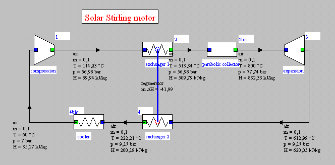
Figure 2.1 : Solar Stirling generator
The objective that we assign the driver is to provide a synthesis of the energies involved in the motor as heat or mechanical power, and calculate the cycle efficiency. Figure 2.2 shows the type of screen that you can imagine.
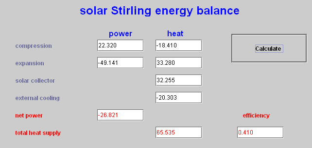
Figure 2.2 : Driver screen
2.2 Computer implementation
2.2.1 Creation of the class, visual interface
To create an external driver, simply subclass extThopt. ExtPilot. Achieving the visual interface poses no particular problem and we do not comment on here.
The constructor must end with a string specifying the code that will identify the driver in the list of those available:
type = "stirling";
It is also recommended to document the class:
public String getClassDescription(){
return "driver for a simple Stirling motor\n\nauthor : R. Gicquel february 2008";
}
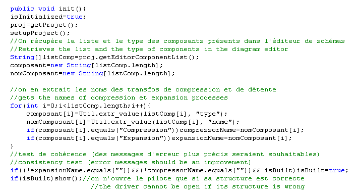
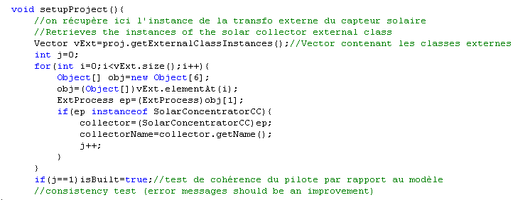
2.2.2 Recognition of components names
It is possible to automatically recognize the names of the various components constituting the model, sorting them by type, which gives the driver greater genericity than if these names are entered as a String in the code. This is done by methods init () and setupProject (), which use methods to access the names of the components of the diagram editor and the list of external classes available (for the external process representing the concentration collector). Caution: if an appropriate diagram is not open in the editor, lists of components are empty and initializations cannot be done properly.
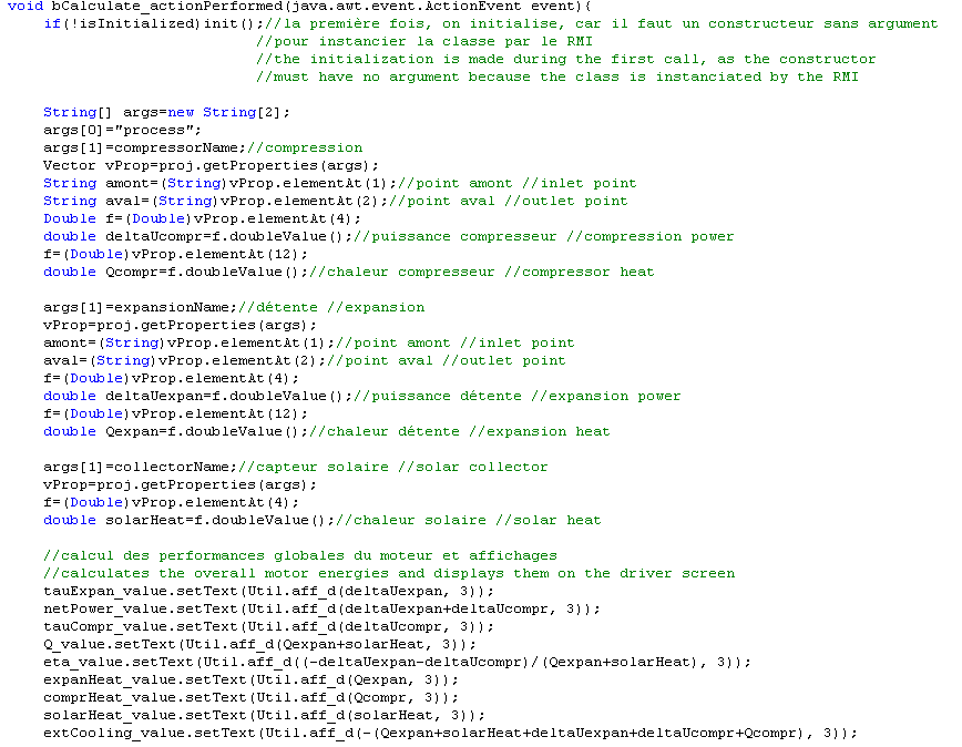
2.2.3 Calculations and display
Once the names of the various components are identified, we access their properties through the Project method getProperties(), which provides all the values you need.
As shown in the code, the execution of an external driver poses no particular problem. This one is particularly simple and simply calculates the energy balances for which the default Thermoptim calculating methods are inappropriate. It would be quite possible to complicate it slightly, so that it could update the simulator to perform the recalculations of the model before establishing the desired balance. We will present further examples involving such features.
2.2.3 Loading a driver
Loading a driver is done by selecting line "Driver frame" of simulator menu "Special". A combo then presents a list of available drivers (Figure 2.3). Select the one you want to load (here "stirling"), then validate.
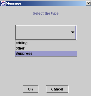
Figure 2.4 : Suppression of a driver
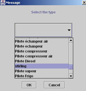
Figure 2.3 : Selection of the driver
When a driver is already loaded, line "Driver frame" shows the screen of figure 2.4, which lets you either return to the driver loaded (line with its name), or select another, or delete the existing without replacing it. Only a single driver may be associated with a project.
3 Technological design
To perform technological design, we have introduced new screens, complementary to those that perform the phenomenological modeling. They can be activated by button "tech. design" placed in the usual screens of the different components.
These new screens allow you to define the geometric characteristics representative of the different technologies used and the parameters necessary to calculate them. For a given component, they obviously depend on the type of technology used.
In the next section, we present a summary of the principles adopted for modeling heat exchangers, compressors, turbines and expansion valves.
3.1 Component technological design
3.1.1 Heat exchangers
The most significant changes relate to heat exchangers, as earlier versions of Thermoptim only determine the UA value, which is the product of the overall heat exchange coefficient U by the exchanger surface A, the two terms not being evaluated separately. To resize a heat exchanger, that is to say calculate its surface, one must first choose a geometric configuration, and second compute U, which depends on that configuration, thermophysical properties of fluids, and operating conditions.
Recall that although the approach we have adopted in Thermoptim is unconventional, it has proved quite fruitful for the study of complex systems: a heat exchanger ensures the coupling between two "exchange" processes, one representing the hot fluid which is cooled, and the other the cold fluid which warms up. It follows that the definition of the exchanger flow patterns and geometry is made at the process level, and not globally.
3.1.1.1 Calculation
The method for calculating heat exchangers in off-design operation is based on the NTU method. When we know the two inlet temperatures and flow rates, an exchanger can be represented by a quadrupole, whose generalized matrix formulation can be expressed in various ways, depending on temperatures known (see chapter 8 (Part 2) of the first edition of the book Energy Systems).
In design mode, the calculation of a heat exchanger is done in three steps:
- knowing the inlet and outlet temperatures and flows of both fluids, we first determine the effectiveness ε, and we deduce UA by the NTU method
- then U is estimated by correlations depending on the exchanger flow pattern and geometry
- the calculation of area A is deduced immediately: A = UA / U
In off-design mode, if we know the inlet temperatures and flow rates of both fluids, the area A of the exchanger and its geometry (flow patterns and technological parameters), the calculation is done in three steps:
- determining U by correlations depending on the flow pattern and geometry of the exchanger ;
- calculating UA, product of U and A, and then NTU
- determining the effectiveness ε of the exchanger by the NTU method, and calculating the hot and cold fluid outlet temperatures
Usually we know the inlet temperatures Tci and Thi of both fluids and their flows mc and mf, and we wish to know the outlet temperatures Tho and Tco when known variables change. If we can determine the value of U, it is possible to calculate R and NTU, to deduce ε and determine Tho and Tco.
But other cases can also be solved: knowing Tci, Tco, mc, mf and U, we can calculate R, then NTU, deduce ε, and determine temperatures Tho and Thi.
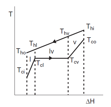
Figure 3.1 : multizone exchangers
The first case could already be calculated by the phenomenological version of Thermoptim: if at least two temperatures are set, the "off-design" calculation mode of the heat exchanger screen allows you to make the calculation by the NTU method. As indicated in section of Volume 2 of the reference manual devoted to heat exchangers, this calculation applies to the study of an heat exchanger already designed for which one seeks to understand how it behaves in off-design conditions. Thermoptim updates the exchanger from the process upstream links, then calculates the downstream temperatures. The points and processes associated are updated based on results.
It is therefore possible to use this calculation mode by changing the UA value as shown in the example discussed Section 4.
3.1.1.2 Multizone heat exchangers
The calculation of multizone heat exchangers is more complex than simple ones, but it relies on the same principle. Let us consider the case of the condenser of a cooling machine whose temperature / enthalpy diagram is shown in Figure 3.1.
The refrigerant leaving the compressor is first desuperheated (Thi-Thv), then it is condensed at constant temperature, and then slightly subcooled (Thl-Tho). In this case, the calculation must be completed for each zone, the surface of the heat exchanger being the sum of the three zone areas. Obviously, the heat transfer coefficients are very different in these three areas.
In off-design mode, the total area remains constant, but its distribution among the three areas varies. A precise calculation is therefore requested to seek the solution that corresponds to the same total area and meets all other thermal and thermodynamic constraints.
3.1.1.3 Geometric setting
The geometric setting of heat exchangers is a difficult subject. Here we just introduce the quantities used, without discussing the reasons for their choice.
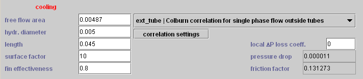
Figure 3.2 : Condensor technological design screen
In order to calculate heat transfer coefficients and pressure drops, two geometrical quantities are particularly important besides the surface of the exchanger: the section Ac devoted to the fluid flow, and the hydraulic diameter dh. When the heat exchange coefficients of the fluids are very different, various devices such as fins can be used to compensate for the difference between their values. This is called extended surfaces, which can be characterized by an area factor f and a fin effectiveness η0.
These four parameters are those which have been chosen in Thermoptim to characterize heat transfer in each fluid. The length of the exchanger is also used for certain calculations such as pressure drops.
In the heat exchanger technological design screen, the following conventions are adopted:
- type configuration (here, "cond") is selected in a combo
- "free flow area" represents the flow area Ac
- "hydr. Diameter is the usual hydraulic diameter dh
- "length" is the length of the exchanger (used for calculating the boiling number Bo and the calculation of pressure drops, not yet implemented in the two-phase case)
- "surface factor" is the surface factor f for large surfaces
- "fin effectiveness" is the fin effectiveness η0
3.1.1.4 Correlations for calculating the heat exchange coefficients
Table 12.1 fluid correlation types
"int_tube" inside tubes Mac Adams single-phase
"ext_tube" outside tubes Colburn (Dittus Boettler) single-phase
"cond" condensation int. tubes Shah/Bivens two-phase
"cond_ext_hor" horiz. cond. ext. tubes B1540 T/I two-phase
"evap" evaporation Gungor Winterton two-phase
"air_coil" air coil Morisot air
"cool_tower" evaporative cooling Colburn moist air
"flooded" flooded generic two-phase
"plate" plate generic single-phase
A major difficulty is the calculation of the overall exchange coefficient U, which depends on the fluid heat transfer coefficients h, by the general formula below. Many correlations have been proposed in the literature, and choosing the one best suited is not always obvious.
The default options offered by Thermoptim are given in the table above. It summarizes the proposed configurations, indicating their type, the correlations used and the type of fluid to which they correspond. It is of course possible to introduce others in additional external classes.
Watch out: for the calculations to be meaningful, it is imperative that the Thermoptim project units are expressed in the SI system, that is to say that the flow is expressed in kg/s. Check out this item, preferably by introducing a specific test in the driver.
3.1.2 Compressors
3.1.2.1 Displacement compressors
A displacement compressor is geometrically defined by its swept volume, and its technological parameters allow calculating its volumetric and isentropic efficiencies, according to its rotation speed, its load factor, and conditions of suction and discharge.
The models implemented in Thermoptim are based on the assumption that the behavior of displacement compressors can be represented with reasonable accuracy by two parameters: the volumetric efficiency λ which characterizes the actual swept volume, and the classical isentropic efficiency ηs.
The calculation of a compressor is made as follows:
- the isentropic and volumetric efficiencies are calculated from the equations above
- if we know the rotation speed, the swept volume and the volumetric efficiency, the volumetric flow can be calculated as:
- knowing the suction density v, we deduce the mass flow:
In design mode, the rotation speed or the swept volume required to provide the desired flow is determined. The calculation is done taking into account the inlet and outlet pressures, and the flow value entered in the compressor flow field.
In off-design mode, the compression ratio allows to determine λ and ηs, which sets the compressor flow and outlet temperature. The sequence of calculations is as follows:
- 1) knowing the inlet and outlet conditions, the compression ratio Pref/Pasp and suction volume v are updated;
- 3) the flow volume is deduced;
- 4) the compressor sets the mass flow and spreads this value to connected components;
- 5) the useful work can then be calculated knowing the isentropic efficiency ηs.
3.1.2.2 Turbocompressors
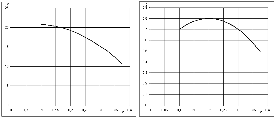
Figure 3.3 Simplified reduced characteristics of a turbocompressor
Turbocompressors can be modeled in several ways. We will use a similitude approach by using two characteristics: the flow factor ϕ, and the enthalpy factor ψ, and we limit ourselves here to the simplifying assumption that their reduced characteristics (ψ, ϕ)and (η, ϕ)) can be represented by simple curves of parabolic type (Figure 3.3).
Other models are presented in the appendix.
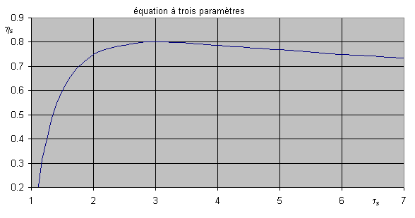
Figure 3.4 : Three parameter equation
3.1.3 Turbines
A turbine is geometrically defined by a section, and its technological parameters used to calculate the isentropic efficiency and the cone constant, depending on the conditions of suction and discharge.
For the isentropic efficiency, it is often possible to retain an equation analogous to the volumetric compressor law.
Note that it is expressed linearly as a function of expansion ratio and its square. Its parameters have the advantage of having a physical meaning
ηlim is the asymptotic value of isentropic efficiency for the high expansion ratio, and ηmax the maximum performance obtained for expansion ratio equal to τmax.
The flow calculation is done using the Stodola rule, which can be expressed as follows, K0 being the cone constant:
Usually, we take k = 1, which corresponds to a quadratic form. If the flow is shocked, this relation is simplified as
Other models are presented in the appendix.
3.1.4 Expansion valves
The technological design of expansion valves is taken into account in a simplified way, because we consider that their dynamics is much faster than that of other cycle components, and therefore they act as regulators.
The only parameter introduced at this level is the superheating value.
3.2 Computer Implementation
The structures of external classes allowing addressing the technological design and off-design operation for the various components of Thermoptim core have a number of similarities with those described in Volume 3, but also some differences that are explained by their characteristics. We will present them in due time.
As major developments have focused on compressors and heat exchangers, they shall be presented here.
3.2.1 General Principles
Firstly, we must ensure consistency with the "phenomenological" Thermoptim classes, which need to perform their calculations in the same way, technological screens being present or not.
This implies in particular that the technological screens should be separate from the "phenomenological" ones.
Then we decided to outsource as much as possible computer implementation so that users can customize the calculations as much as they want. Indeed, it is virtually impossible on the one hand to find completely generic formulations given the multiplicity of technological options, and on the other hand to develop algorithms robust enough to solve the corresponding sets of equations. By outsourcing these classes, users can relatively easily adapt them to the specific problems they face.
We therefore limited ourselves to make available a working infrastructure which should significantly facilitate their task.
In principle, we believe that calculations of technological design and off-design should be performed in external classes, so that those we have built into the core are essentially devoted to allow communication between it and external classes.
Indeed, the core objects being not directly accessible from the outside, the information exchange needs to be made following rules that are a little binding. We sought to make it as flexible and user-friendly as possible, further than was possible using communication methods presented in Volume 3. The methods we have implemented for this purpose are documented in the appendix.
3.2.2 Structure
In the component screens, button "tech. design" provides access to the technological setting screen. The technological setting screens can be managed centrally from the menu line "Technological design screens" of the "Technological Design" simulator menu.
The TechnoDesign class is the superclass of the technological setting screens. It is subclassed by screens specific to each component type, according to the principle presented Section 2.3 of Volume 3.
Method makeDesign() of TechnoDesign actually implements the technological design.
In TechnoDesign, classes derived from JPanel allow to change the settings according to the technological choices made.
External mother classes representative of the main types of components have been prepared. They are intended to be subclassed by users depending on their requirements.
The only way to instantiate the TechnoDesign recognized by the core is to do it in an external driver, then load them in Vector vTechno of this driver. Therefore, they become visible from the core and may be associated with their components. This choice means that the external drivers play a major role in the technological design and off-design operation.
Saving technological settings is done by the driver at the end of project files. The last line must end with a newline ("\ n"). Some TechnoDesign may require several lines (it is the case for heat exchangers, which use one for the overall results, and one for each fluid, as well as for thermocouplers who use two).
All technological design classes inherit from class extThopt.ExtTechnoDesign which has a JPanel called JPanel1, in which is designed the GUI.
It has two constructors :
public ExtTechnoDesign(Projet proj, String componentName, PointThopt amont, PointThopt aval){
}
public ExtTechnoDesign(Projet proj, String componentName){
}
The first assumes that the user defines his own upstream and downstream PointThopt, while the latter instantiates them automatically from the project properties, giving it greater genericity.
The PointThopt presented in appendix, which are kinds of external clones of the core points, give access to upstream and downstream states. The constructor instantiates a CorpsThopt (see Appendix) to help perform some thermodynamic calculations.
Method updateDeltaH() is used to update the enthalpy balance of the component. This class also has a method getFlow(), which allows to update the flow from the core.
We comment here two implementation examples, related to compressors and heat exchangers, which are used in the examples in this volume. Others are constructed similarly.
3.2.2.1 Displacement compressors
The VolumCompr class includes:
- method setupPanel(), which builds the JPanel in the technological screen GUI, which is not detailed here. This interface allows to enter the necessary settings.
- generic methods for calculating the isentropic efficiency and flow, and display them on screen.
The constructors are:
public VolumCompr(Projet proj, String compressorName, PointThopt amont, PointThopt aval){
super(proj, compressorName, amont, aval);
this.compressorName=componentName;
setupPanel();
}
public VolumCompr(Projet proj, String compressorName){
super(proj, compressorName);
this.compressorName=componentName;
setupPanel();
}
They call for ExtTechnoDesign constructors, then, in order to use the specific name of compressorName, they identify it with componentName, and finally, they build the JPanel.
This class defines in particular the two methods for calculating isentropic and volumetric efficiencies:
double getRisentr(){
K1=Util.lit_d(K1_value.getText());
K2=Util.lit_d(K2_value.getText());
K3=Util.lit_d(K3_value.getText());
R1=Util.lit_d(R1_value.getText());
R2=Util.lit_d(R2_value.getText());
double r_compr=aval.P/amont.P;
double risentr=0.5;
if(R1*R1+R2*R2==0)risentr=K1+K2/r_compr+K3/r_compr/r_compr;//3 parameter equation
else risentr=K1+K2*(r_compr-R1)*(r_compr-R1)+K3/(r_compr-R2);
risentr_value.setText(Util.aff_d(risentr,7));
return risentr;
}
double getLambdaVol(){
a0=Util.lit_d(a0_value.getText());
alpha=Util.lit_d(alpha_value.getText());
double r_compr=aval.P/amont.P;
double lambda= a0-alpha*r_compr;
display_value.setText(Util.aff_d(lambda,7));
return lambda;
}
Saving the parameter values is done using method saveCompParameters(), which, as we said above, should end with a line feed character.
public String saveCompParameters(){
String h="alpha_value="+alpha_value.getText()+tab
+"K1_value="+K1_value.getText()+tab
+"K2_value="+K2_value.getText()+tab
+"K3_value="+K3_value.getText()+tab
+"R1_value="+R1_value.getText()+tab
+"R2_value="+R2_value.getText()+tab
+"N_value="+N_value.getText()+tab
+"Vs_value="+Vs_value.getText()+tab
+"Device_number="+deviceNumber_value.getText()
+"\n";//retour à la ligne impératif //compulsory line feed
return h;
}
3.2.2.2 Heat exchangers
A notable difference between a heat exchanger and a compressor is that the second is a single component, while the first is a thermal coupling between two exchange processes. However, the thermal coupling equations are the same for all types of heat exchangers that Thermoptim can calculate, with one exception: multizone exchangers often occur as exchange areas in which liquid and vapor two-phase boundaries are evolving over time. It is therefore impossible to assign to each a fixed area: they must be continually recalculated, even if the total area is known.
The heat exchanger TechnoDesign is called TechnoHx. In design mode, it calculates U and proposes a value of the exchanger surface A. It performs its calculations by estimating all thermophysical properties of fluids. Chapter 35 (Part 5) of the book Energy Systems specifies how they are determined.
The TechnoDesign for exchange processes is TechnoExch. It also allows to calculate the pressure drop when methods are implemented. To ensure a seamless calculation between the two processes and the heat exchanger it connects, TechnoHx makes a direct call to both TechnoExch associated, which are loaded on its screen. The process TechnoExch of an exchanger are thus not instantiated independently of the TechnoHx.
Different flow patterns have been introduced: they all inherit from FlowConfig and are selected in the TechnoExch screen. They make the calculation of thermophysical properties and the Nusselt number, especially for multi-zone heat exchangers.
In summary:
- TechnoHx introduces the exchanger surface, designs it (makeDesign ()), manages displays of calculations of thermophysical properties and instantiates cold and hot TechnoExch
- the cold and hot TechnoExch make the calculations of thermophysical properties and manage FlowConfig through a ComboBox. The JPanel for TechnoExch appears in the TechnoHx window.
- FlowConfig implement the correlations for calculating the exchange coefficients and pressure drop
- the SettingsFrame of a FlowConfig allow one to modify its settings.
The TechnoHx class constructor is as follows. It differs from the previous one because of the special structure of the class. It begins by retrieving the names of hot and cold process’s that it matches, instantiates four PointThopt to get access to inlet and outlet states of both fluids, and builds their technological displays. He then tells each what is his counterpart. Finally, it configures the screen.
public TechnoHx(Projet proj, String hXname, PointThopt amontHot, PointThopt avalHot, PointThopt amontCold, PointThopt avalCold){
this();
this.proj=proj;
this.hXname=hXname;
String[] args=new String[2];
args[0]="heatEx";
args[1]=hXname;
Vector vProp=proj.getProperties(args);
hotFluid=(String)vProp.elementAt(0);
coldFluid=(String)vProp.elementAt(1);
this.amontHot=amontHot;
this.amontCold=amontCold;
this.avalHot=avalHot;
this.avalCold=avalCold;
techc=new TechnoExch(proj, this, hotFluid, amontHot, avalHot);
techf=new TechnoExch(proj, this, coldFluid, amontCold, avalCold);
techc.setOtherTechnoExch();
techf.setOtherTechnoExch();
JLabCompName.setText(hXname);
hotName.setText(hotFluid);
coldName.setText(coldFluid);
setupPanel();
setupTechHx();
}
The class then implements a variety of methods to perform thermodynamic calculations.
The TechnoDesign constructor of "exchange" processes is similar to that of the compressor. There are actually three variants, their signatures differing because of the need for them to know whether they are connected to a heat exchanger (TechnoHx), a thermocoupler (TechnoT) or are isolated.
public TechnoExch(Projet proj, TechnoHx tHx, String exchangeName, PointThopt amont, PointThopt aval){
this(proj, exchangeName, amont, aval);
this.tHx=tHx;
}
public TechnoExch(Projet proj, String exchangeName, PointThopt amont, PointThopt aval){
super(proj, exchangeName, amont, aval);
this.exchangeName=componentName;
setupPanel();
JLabCompName.setText(exchangeName);
fc=new IntTubeConfig(this);
setupListeConf();
}
TechnoExch being the technological design class of exchange processes, it plays an essential role in the study of heat exchangers.
Global variables are defined as follows:
boolean diph;
TechnoHx tHx;
TechnoExch otherTe;
TechnoTC tTc;
public FlowConfig fc;
SettingsFrame sf;
String[]listeConf;
diph allows one to specify that the calculation of exchange coefficients must be done in two phase mode.
tHx is the calling TechnoHx instance when TechnoExch is part of a heat exchanger.
otherTe is the second exchanger TechnoDesign in this case.
tTc is the calling TechnoTC instance when TechnoExch is part of a thermocoupler.
fc is the FlowConfig defining the flow pattern.
sf is the setting screen for the FlowConfig correlation coefficients
listeConf is a list of flow patterns available that allows the user to specify the type of flow pattern in which the fluid flows, and therefore the equations to be used to calculate the heat exchange coefficients.
Method setupListeConf() dynamically builds the FlowConfig list when loading Thermoptim, depending on external classes that define them. The codes defining these flow patterns and their description are loaded into a dropdown list so the user can make his choice. In case of doubt, if the list is too narrow, you can display the corresponding parameter by clicking on "correlation settings, which allows you to read the entire description (see Figure 3.11).
The constructor of the superclass is given below. It combines to the FlowConfig the TechnoExch who called on it, and initializes values needed to calculate the Nusselt number.
public FlowConfig (TechnoExch te){
this.te=te;
C1=0.023;a_Re=0.8;b_Pr=0.4;c_Visc=0.14;RR=0.001;
te.JLabel13.setText("length");
otherTe=te.otherTe;
}
To add another configuration, simply subclass FlowConfig and give it a reference that is not already used, then place the class in extThopt.zip or extUser.zip. It will automatically be included in listeConf.
In two-phase regimes, the calculation of pressure drops can be very complex, especially since it is necessary to start by determining the lengths of the different areas of the exchanger. Several correlations were implemented in early 2021.
Other correlations are also available, both for two-phase pressure drops and for the Nüsselt calculation.
Pressure drops are calculated in FlowConfig as follows.
In laminar flow, the losses are proportional to the flow rate and fluid viscosity: f = 64/Re.
For smooth tubes, f is given by the Blasius formula (f = 0,316 Re-0,25) if Re < 30 000, or by the following formula (0,0032 +0,221 Re-0,237) for higher values of Re.
For rough pipes in turbulent regime (Re> 2100) the friction coefficient is given by the Colebrook equation:
=
= Absolute roughness of pipe
We can show that the implicit equation giving f can be approximated by:
=
The settings of SettingsFrame allow to calculate the pressure drop with the Colebrook formula if this option is selected, or with the Blasius one otherwise.
In two-phase system, pressure drop calculation of can be very complex, in particular because the different areas of the heat exchanger must first be determined.
In the vapor-liquid equilibrium zone, we use the approximate formula for the nuclear steam generator proposed by Herre and Gallori adjusted to take account of an nonzero quality inlet.
∆Pdiff = ϕ ∆Pliq
ϕ = [][]-0,2
The pressure drop is thus calculated from the saturated liquid state using this factor.
3.2.3 Technological and simulation screen
A technological and simulation screen has been added to the simulator. It is accessible from line "technological design screens" of the "Technological design" simulator menu (Figure 3.5), or by typing Ctrl T. It has two main tables placed in its left side. The upper one provides access to all TechnoDesign instantiated by the driver and loaded into Vector vTechno. Double-clicking on a line opens the TechnoDesign selected. The one below provides quick access to certain Thermoptim points or processes described as observed because we want to observe their thermodynamic state.
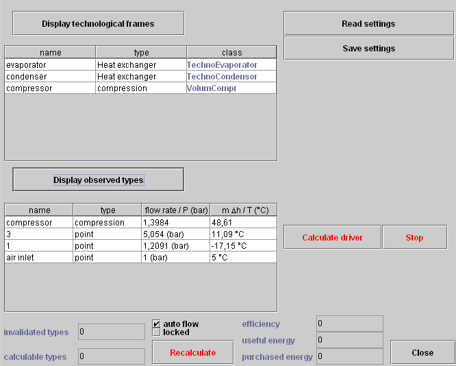
Figure 3.5 : Overall technological design tool screen
Buttons and displays at the bottom of the screen facilitate automatic recalculation, which can be triggered without returning to the simulator main screen.
The two buttons "Calculate the driver" and "Stop" can start and stop the calculations of the driver without blocking access to Thermoptim (it runs in a separate thread), which presents the advantage that it is possible to access all the software functions while it conducts operations coded in the driver. Button "Stop" can stop the calculations if necessary.
To use this feature requires that the calculation method of the driver be named calculatePilot(). Obviously, it is recommended not to make setting changes while the driver runs, to avoid interference.
The two buttons at the top right, "Save Settings" and "Read Settings", allow you to save a technological setting made by a driver, and read it by a similar one, which avoids having to re-enter all the values each time you change driver.
3.2.4 Generic driver for creating technological screens
We show in Section 4 how to create screens by building technological drivers, which requires a minimum of programming. This work is imperative when you want to perform off-design calculations, because it is then necessary to take control of Thermoptim recalculation engine.
However, if you simply want to make the technological design of a project that only implements core Thermoptim components, it is possible to automatically create technological screens using the generic driver that we will briefly present. This avoids having to program one.
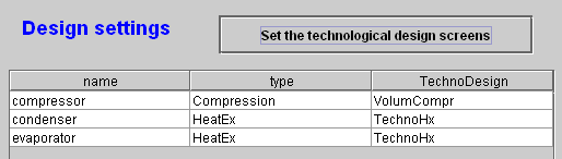
Figure 3.6 : Generic driver screen (default initialization)
Open the Thermoptim project and load the generic driver by choosing the one whose title is "generic techno design pilot", in the list of drivers, then click "Set the technological design screens" (Figure 3.6). The list of components for which there are technological screens is displayed in the table with their name, type and technological screen class name instantiated by default: VolumCompr for the compressor and TechnoHx for the heat exchangers in Figure 3.6 example.

Figure 3.7: Generic driver screen after selection
In this example, this initial setting is suitable for the compressor, but not for heat exchangers: the condenser should be modeled by class TechnoCondensor, and the evaporator by TechnoEvaporator.
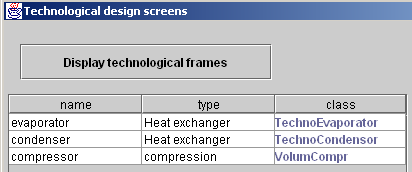
Figure 3.8 : Technological screen window
To change a component’s TechnoDesign class, select its line and double-click. A message asks you to confirm your choice, then displays a list of available classes. Choose the one you want and confirm. After modifying the two heat exchanger classes, you get the screen shown in Figure 3.7.
You can then access the screens of these technological components either from their own screens (button "tech. design") or from the technological and simulation window presented in the previous section. It can be opened from the simulator screen (Figure 3.8).
3.3 Example of heat exchanger design
3.3.1 Presentation and results
Consider a tube and fin heat exchanger intended to cool about 0.66 kg/min of air leaving a compressor at 5 bars and 275 °C with a flow rate of 1.17 kg/min of cold water passing through a coil of two parallel tubes. The diameter of the tube is 15 mm, and its thickness 1.5 mm. The spacing between the fins is 3 mm.
The exchanger can be easily modeled in Thermoptim.
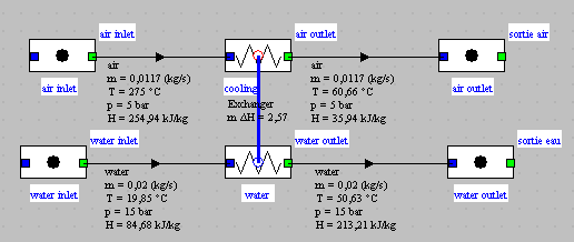
Figure 3.9 : Example synoptic diagram
To design the heat exchanger, we set an effectiveness of 0.84.
Using the Thermoptim technological design screens, it is possible to calculate the overall heat exchange coefficient and to deduce the area required to transmit the desired power.
This requires determining the hydraulic diameter dh and flow section Ac of both fluids.
Inside the tubes, dh is given, and the calculation of Ac is very simple: it is equal to the product of the number of tubes by the tube section. Outside the tubes, the calculations are somewhat more complicated. dh is equal to 4 times the flow area by the wetted perimeter and Ac is the cross-sectional area available to the air.
We assumed that the fins multiplied the exchange surface by 4, their effectiveness being equal to 0.8.
These values must be entered in the heat exchanger technological design screen. After some trial and error, we obtain a setting similar to that of figure 3.11.
The driver can then calculate the area needed, which is here equal to 0.067 m2, the exchange coefficients being 669.3 W/m2/K on the air side, and 759.1 W/m2/K on the water side, leading to a global coefficient equal to 355.7 W/m2/K.
The heat exchanger will be comprised of two 90 cm tubes arranged in a 3 layer coil and traversing steel sheets separated from each other by 3 mm, with a total extended area of 0.31 m2.
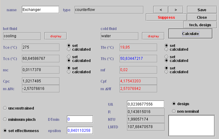
Figure 3.10 : Heat exchanger screen
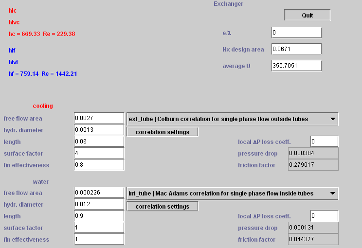
Figure 3.11 : Heat exchanger technological design screen
As we said in the previous section, it is here possible to use the generic driver to build this technological screen. However, as this simple example lends itself well to a first driver presentation, we explain below how to create one.
3.3.2 Driver implementation
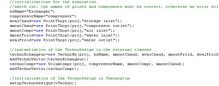
The driver class is called AirExchangerDriver. Its interface is simple and classical, we do not break it here.
3.3.2.1 Initializations
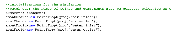
For the name of the exchanger, we could use the Project method getHxList(), but it requires the diagram to be loaded in the diagram editor. To avoid this constraint, it can be declared in the code.
For the other initializations we use PointThopt instances, which are kind of clones of Thermoptim core points giving easy access to their values. Four of these objects are instantiated, representing the inputs and outputs of the two fluids. Here we have their names entered by hand, but it would be possible to automatically recognize them.
The screen technology is then instantiated and the Vector vTechno built :
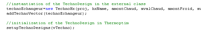
The last line initializes the TechnoDesign when opening an existing project file or loading the original driver. Without it, it does not appear in the TechnoDesign list of the technological and simulation screen of Figure 3.5.
3.3.2.2 Calculations
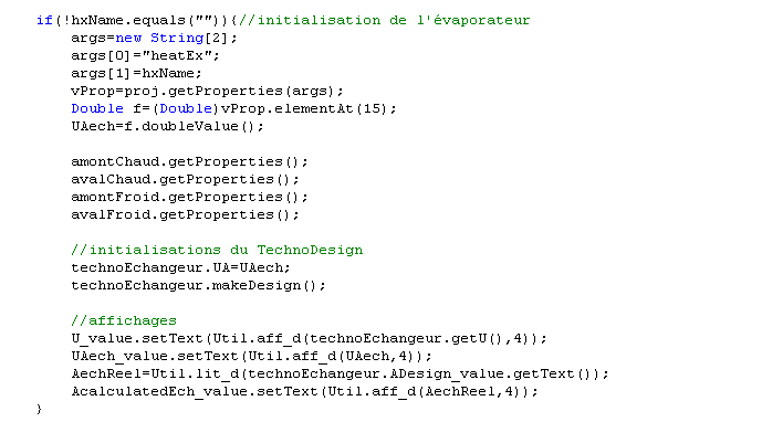
The calculations here are very simple: using Project method getProperties(), the driver retrieves the values of UA and ∆H. The exchanger is then calculated by method makeDesign() and the results are displayed on the screen.
3.3.2.3 Backup
In this example, there are no particular backups to make considering constant thermal resistance of fouling. Standard methods for the backup of technological parameters will do.
Two ExtPilot methods, transferTechnoData() and setupTechnoDesigns(), are used to initialize the driver and technological screen while opening an existing project file.
The first method groups all lines in the project file on technological screens and loads them in the driver until it is built, and the second decodes these lines to perform its initialization, passing the values to the standard TechnoExch methods, which in turn call the FlowConfig ones.
The last line of setupTechnoDesigns(), proj.bindTechnoDesigns(vSettings), is used to link the TechnoDesign used by the driver with the core components, so they can be displayed from their screens and from the tables of the main technological and simulation screen.
4 Off-design
The computer structure developed in order to perform technological design also allows to analyze the off-design operation of models created with Thermoptim.
This type of analysis includes, however, additional difficulties: they require the modeler to be able first to write the set of equations describing the coupling existing between the various components of the system studied, and second to find an appropriate resolution algorithm.
The cases we have treated have shown us that there are two major additional challenges:
- the first concerns the development of physical phenomena equations. The behavior of the different components must be analyzed carefully and modeled correctly, which may be far from simple. We propose in the examples posted on the Thermoptim-Unit portal a number of models, but variants are also possible, and we have not covered all interesting cases;
- the second corresponds to the resolution, usually numerical, of the model equations, which requires first to find a suitable algorithm, and second to initialize it properly.
As our intention is primarily focused on applied thermodynamics, we mainly concentrated on the first difficulty. Numerical tools that we offer use either Thermoptim own libraries, to perform simple searches by dichotomy, or generic, like minPack, which is a set of classes allowing to make nonlinear optimization, in particular seek the solution of systems of equations. It will be presented in Section 4.3.
We will start initially by treating a simple example that does not pose any problem of numerical resolution and explain the code of the driver class.
4.1 Example
To illustrate the ability of Thermoptim to perform off-design calculations, we will study the behavior of a volumetric air compressor that fills a compressed air storage volume at variable pressure. The compressed air is cooled before storage with a water exchanger of the kind just presented.
The system can be easily modeled in Thermoptim and leads to a diagram like Figure 4.1, which differs from that studied in the previous example by adding the compressor.
The technological design screen of the compressor is given in Figure 4.2. The heat exchanger is similar to the previous one. They correspond to the physical models presented in Section 3.1 of this manual.
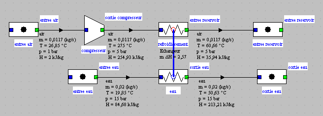
Figure 4.1 : Example of compressor cooling
Note, as we have not yet said that double-clicking the component name (here "compressor" located under the small arrows in the upper right) provides access to its phenomenological thermodynamic screen.
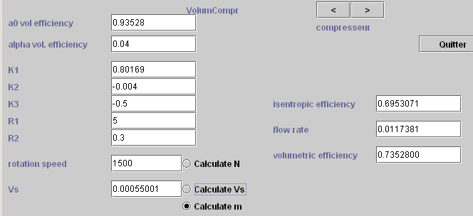
Figure 4.2 : Compressor screen
4.1.1 Results
Once the driver made, it is very easy to make the compression ratio vary in order to get the evolution of the main variables when the pressure of the tank changes. They can be processed with the Thermoptim simulation files Excel post-treatment macro presented in Volume 1 of the reference manual. Simply save the project file under a different name after each simulation, then load these files into the macro and extract the interesting values.
Figure 4.3 shows, as a function of the storage pressure, changes in the isentropic efficiency and compression work, intake air flow, temperature of air entering the tank, exchanger load and U value.
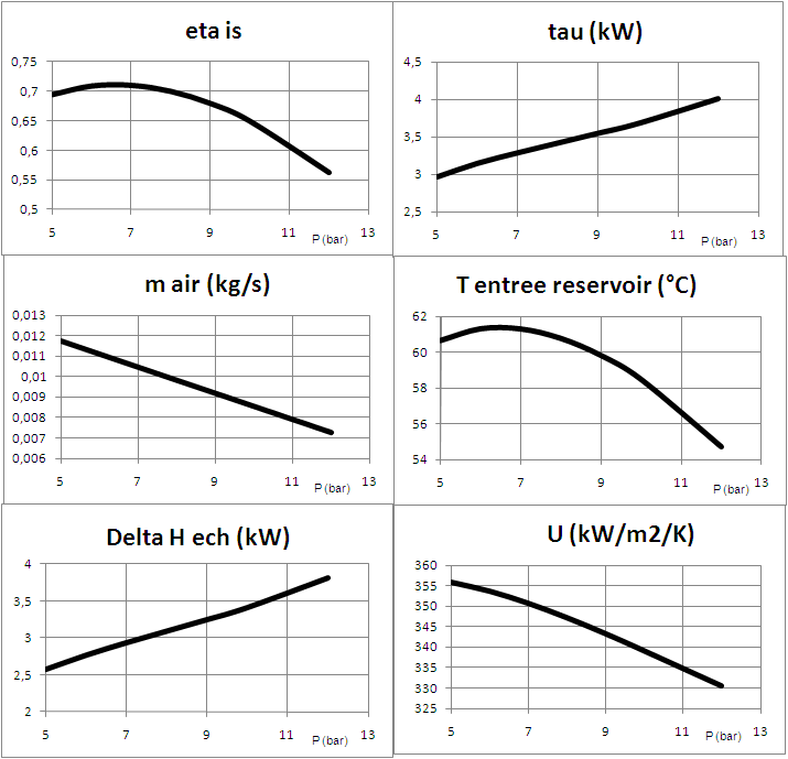
Figure 4.3 : Simulation results
4.1.2 Driver implementation

Figure 4.4 : Driver screen
The driver class is called VsCompressorDriver and its type is "Vs compressor driver". Its interface being simple and classic, we do not break it here.
The driver screen is shown in Figure 4.4.
To write the relevant class, we start from the exchanger driver one, and complement it on two points:
- first by instantiating and initializing the compressor technological screen, as for the heat exchanger;
- second by introducing a button "Calculate" and defining calculations and changes in the simulator settings which should be carried out when the downstream pressure varies.
4.1.2.1 Initializations
During initialization, after the PointThopt and the two TechnoDesign have been constructed, the compressor swept volume Vs required to obtain the desired flow is determined on the basis of technological screen settings.

4.1.2.2 Calculations
The calculations are made as follows:
- first initialize the swept volume and update the compressor output pressure
- calculate its volumetric and isentropic efficiencies, determine the mass flow rate transferred and propagate it upstream and downstream
- recalculate the compressor and its downstream process, knowing that, set as isobaric, it propagates the new pressure
- update exchanger inlets and outlets and then recalculate the off-design operation after having updated the air heat flow rate
- update the simulator and recalculate the project several times to ensure the stabilization of values.
This example illustrates even better than its predecessor the interest of the PointThopt used to communicate between the driver and the simulator. The syntax of updates is much more readable than when using only Project methods getProperties() and updatePoint().
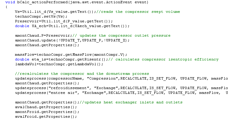
The calculation of the compressor is done by methods getRisentr() and getLambdaVol() introduced previously. Method updateprocess() modifies the compressor flow and isentropic efficiency and then recalculates it. Its outlet point, called here "amontChaud" because it corresponds to the heat exchanger upstream hot fluid is then updated.
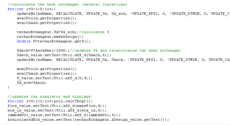
The calculation of the heat exchanger is made as follows: first we make a calculation using method updateHx() by setting the UA value read at the screen, UA_ech (heat exchanger is set for the off-design calculation mode so that the value of UA is taken into account). This calculation allows the exchanger to initialize the new operating conditions.
We then call method makeDesign() of TechnoDesign, which updates the value of U. The real UA is obtained by multiplying the new U with the initial value of A (AechReel), which allows the exchanger to recalculate properly.
Since U depends on the average temperatures of fluids, and therefore those of outlets, we iterate five times the calculations to ensure proper stabilization, resetting each time UA_ech.
4.1.2.3 Backup
Backups and updates on project loadings are similar to those of class PiloteEchangeur. Method setupPilot() has been supplemented to reflect the existence of the compressor.
4.2 Using the model to simulate the filling of a compressed air storage
The results obtained can be used to simulate the filling of a compressed air storage. For this simulation, we develop a second model, solved with Excel, with the following equations:
- The air mass M contained in the storage is equal to the initial mass plus the integral of the mass flow
- the internal energy U is equal to the initial internal energy plus the integral of the product of the flow by the enthalpy of air leaving the cooler, less the integral of losses by convection with ambient air
- the storage temperature is inferred from its internal energy
- the pressure is then calculated by the ideal gas law.
To find the flow and the enthalpy of the air stored, just make polynomial regressions from Thermoptim simulations.
To find the flow, the compression work and the temperature of the air entering storage, simply do polynomial regressions from Thermoptim simulations. Equations obtained, function of the compression ratio r, are:
= - 0.0006 r + 0.0149
τ = 0.0019 - 0.0484 + 0.5322 r + 1.2806
Tair = 0.01 - 0.4735 + 4.9142 r + 46.699
The look of the results is given below, for a half m3 storage (diameter 80 cm, length 1 m), powered by a compressor of Vs = 0.525 l swept volume. The pressure and temperature in storage, its mass and the compressor workload are shown in figure 4.5.
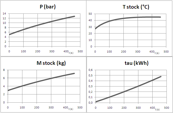
Figure 4.5 : Filling the compressed air storage
This example has taught you how to write a driver to simulate the behavior in off-design operation regime of a relatively simple thermodynamic system. For further investigation, we advise you to study the code of a cooling machine driver available on the Thermoptim-UNIT portal.
4.3 Use of minPack solver for solving systems of nonlinear equations
In many cases, the equations describing the off-design behavior of an energy system are nonlinear, so that their resolution is a difficult problem, particularly when the number of unknowns is high.
4.3.1 Presentation of minPack
Based on the method of Levendberg-Marquardt minPack is a set of algorithms developed in Fortran and then translated to Java. This method combines the Gauss-Newton and gradient descent methods. Its main interest is to be very robust and not to require initialization by an approximate solution.
Note that minPack is actually a set of minimization algorithms that can be used to find the minimum of the L2 residuals ||F(X)|| a set of m non-linear equations in n unknowns F( X).
When n is equal to m, minPack can be used to solve the system of equations F(X) = 0, or at least seek a vector X that is as close as possible to the solution.
You can also use minPack to identify a set of n parameters to fit a nonlinear equation on a set of m data.
4.3.2 Implementation of minPack
The set of classes required is included in library extBib.zip which must be declared in the classpath.
The implementation of Java minPack is done using an interface called optimization.Lmdif_fcn, which forces the calling class to have a method called fcn().
This method fcn() receives as key arguments a vector (array x[n]) containing the variables and a vector (array fvec[m]) referring to residues of the functions one seeks to set to zero. As we have indicated, number m may exceed the number of variables n, but it must be the same if we seek the solution of a system of equations.
Guiding the algorithm is done in practice by playing on two accuracy criteria, one on the residuals, and the other on the accuracy of the calculation of partial derivatives, estimated by finite differences.
4.3.3 Example
To illustrate the use of minPack, we have written a test class called TestMinPack, which solves the equation system corresponding to the intersection of a circle and a straight line. The code is as follows:
int info[] = new int[2];
int m = 2;//système de deux équations / / system of two equations
int n = 2;//à deux inconnues / / with two unknowns
int iflag[] = new int[2];
double fvec[] = new double[m+1];//vecteur des résidus / / vector of residuals
double x[] = new double[n+1];
double residu0;//norme L2 initiale
double residu1;//norme L2 finale
System.out.print("\n\n\n\n\n problem dimensions: " + n + " " + m + "\n");
//initialisation des inconnues / / Initialization of the unknowns
x[1] = 1;
x[2] = 0;
iflag[1] = 0;
testMinPack.fcn(m,n,x,fvec,iflag);//premier appel pour calcul norme L2 initiale / / first call for calculating initial L2
//norme L2 initiale
residu0 = optimization.Minpack_f77.enorm_f77(m,fvec);
testMinPack.nfev = 0;
testMinPack.njev = 0;
double epsi=0.0005;//précision globale demandée sur la convergence / precision required on the overall convergence
double epsfcn = 1.e-6;//précision calcul des différences finies / / precision calculus of finite differences
//appel à minPack / / Call for minpack
optimization.Minpack_f77.lmdif2_f77(testMinPack, m, n, x, fvec, epsi, epsfcn, info);
//norme L2 finale
residu1 = optimization.Minpack_f77.enorm_f77(m,fvec);
//affichage des résultats / / Display results
System.out.println("\n Initial L2 norm of the residuals: " + residu0 +
"\n Final L2 norm of the residuals: " + residu1 +
"\n Number of function evaluations: " + testMinPack.nfev +
"\n Number of Jacobian evaluations: " + testMinPack.njev +
"\n Info value: " + info[1] );
System.out.println();
System.out.println("precision: \t" + residu1);
for(int i=1;i<=n;i++){//affichage de la solution
System.out.println("x["+i+"] \t" + x[i]);
}
function fcn is defined as follows:
public void fcn(int m, int n, double x[], double fvec[], int iflag[]) {
if (iflag[1]==1) this.nfev++;
if (iflag[1]==2) this.njev++;
fvec[1] =x[1]*x[1]+x[2]*x[2]-1;
fvec[2] =3*x[1]+2*x[2]-1;
}
The results obtained are as follows, for initialization x[1] = 1, x[2] = 0 :
problem dimensions: 2 2
Initial L2 norm of the residuals: 2.0
Final L2 norm of the residuals: 2.39665398638067E-10
Number of function evaluations: 6
Number of Jacobian evaluations: 10
Info value: 2
precision: 2.39665398638067E-10
x[1] 0.7637079407212384
x[2] -0.6455619110818576
for initialization x[1] = 0, x[2] = 0 :
problem dimensions: 2 2
Initial L2 norm of the residuals: 1.4142135623730951
Final L2 norm of the residuals: 3.853333208070353E-10
Number of function evaluations: 9
Number of Jacobian evaluations: 12
Info value: 2
precision: 3.853333208070353E-10
x[1] -0.3021694793631984
x[2] 0.9532542190447976
This example illustrates on the hand how minPack can be used, but also the importance of initializing well the problem. In our case, the problem has two solutions, but the algorithm is satisfied with the first that it finds, which is the closest to the starting value.
5 Methodology for identifying component parameters
When attempting to perform off-design calculations, two major methodological difficulties are obtaining experimental data usable and model parameterization of components selected. We assume in what follows that we have well validated measured data. Experience shows that methods presented here can help diagnose data inconsistencies if any.
This methodological section discusses component parameter identification. To facilitate this delicate task, Thermoptim has been equipped with special screens accessible from menu "Technological design" of the simulator screen. These screens allow to:
- import experimental data in project files;
- automate simulations on a series of project files;
- perform sensitivity analysis on the influence of parameters involved in the correlations used to size heat exchangers.
It is indeed first necessary to enter the available experimental data in the form of Thermoptim project files. In general, it is best to begin by identifying parameters of the different components separately and then study the behavior of the coupled system. Procedures presented here allow to automate the creation of project files relating to various processes and evaporators, which require special treatment.
Once we have generated a set of Thermoptim project files consistent with experimental data, the identification process is to try several sets of values of component design parameters, to find one that is consistent with both measured values and what is known about the geometry and the technology of devices tested. To facilitate this process, two families of monitors have been created. The first allows for generic changes to project files and launches a series of simulations, which can then be exploited using the Thermoptim file after-processing Excel macro. The second is specific to the setting of heat exchangers.
5.1 Experimental data import
We must first create a project file of the component, setting it as well as possible on the geometry, and we also usually rather create its diagram. As noted below, the setting will be made on the basis of the names of points and processes. To facilitate comparison with experimental results, it is preferable to adopt the same conventions in the Thermoptim model and in the test bench.
Line "Import experimental data" of menu "Technological design" displays a screen that enables you to import experimental data in a Thermoptim project file (Figure 5.1.1). This screen gives access to three menus and buttons, whose functions are equivalent.
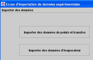
Figure 5.1.1: Data import screen
The principle is the same for all buttons:
- A project must have been loaded prior to importing data;
- A properly structured data file (Figure 5.1.2) is read. Each row contains the values on the one hand of temperatures and pressures of different points, and on the other hand flow-rates of different processes of the project. When reading a line, points and processes are updated, and specific calculations are made possible;
- The project file is then saved under a new name in directory "ModifiedProjects", and the next line is read.
5.1.1 Point and process data import
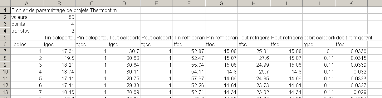
Figure 5.1.2: Experimental data import file
Figure 5.1.2 shows the structure of a default data file for button "Import data for points and processes":
- the first row is not read;
- the second contains in second column the number of values to read;
- the third gives the number of points (np);
- the fourth gives the number of processes (nt);
- the fifth is not read: it allows, if desired, to document the contents of each column;
- The sixth allows Thermoptim to recognize the names of points and processes that need to be modified;
- the following lines are data lines.
The structure of the data lines is:
- the first column contains the string of characters that, when saving the imported data will be concatenated to the name of the project initially loaded;
- the np series of next two columns provide the values of temperatures (°C) and pressures (in bar) of points to be imported (the name of the point to change is that which appears same column in line 6; if no point of that name exists in the project import does not occur);
- the nt series of next two columns provide the values of the flows of different processes to import (the name of the process to change is that which appears same column in line 6; if no process of that name exists in the project, import does not occur).
In the example of Figure 5.1.2, after reading line 7, point "tgec" is set at a temperature of 17.61 °C and 1 bar pressure, and flow from process " tgec" is 0.1 kg/s. If the name of the project file initially loaded is "my_project_.prj", the corresponding project file has the name "my_project _1.prj".
5.1.2 Case of an evaporator
Most of the time, when making measurements on an evaporator, we know the inlet and outlet pressures and temperatures of the two fluids and their flow, but ignore the quality of the refrigerant at inlet. The enthalpy balance of the exchanger, however, can be estimated. Button and menu "Import evaporator data" allow, as the previous, for setting project files, plus calculating an inlet quality and updating pressure factor, used to take into account a pressure drop.
To avoid confusion, the import file must have a special structure (Figure 5.1.3): it should have only two processes, the refrigerant ("refrig"), and the coolant ("mg1"), and the four inlet and outlet points of the two processes (in any order, but appearing before processes in the lines of the file). The value of the pressure factor is saved in the refrigerant TechnoDesign: if we do not want it, we must either enter the same value of pressure at the input and output data file, but this induces a small bias or load the pressure factor, then put it to 1 before simulation using the procedure for amending project files explained Section 5.2.1.
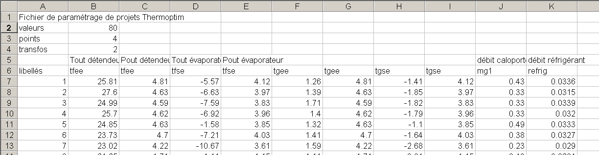
Figure 5.1.3: Evaporator import file
When generating project files (which are stored in directory "ModifiedProjects"), a text file called "evap.txt" is created. It contains in the order of data import file, the values of the refrigerant boiling temperature at the inlet pressure, quality, and cooling capacity.
5.2 Automatic simulation of series of project files
Identifying Thermoptim project parameters leading to better reconstruction of experimental values is to seek the values of these parameters allowing, during simulations, to obtain the smallest gap between the numerical results and measurements and technological data.
To do this we begin, through import data procedures presented section 5.1, by building as many project files as there are experimental measurements, by setting the input variables such as pressures and temperatures at the component inlet.
Once this set of project files is created, the identification process is:
- changing, for each of them, one or more parameters, such as a hydraulic diameter or a free flow area in the case of a heat exchanger;
- then simulating them in Thermoptim;
- finally comparing the results with experimental measurements.
Successively modifying by hand these parameters quickly becoming tedious, it is necessary to automate this process. Line "Automatic simulations" gives access to a screen that has two buttons to initiate actions, and a stop button if something goes wrong.
Button "Modify and save" can perform a series of changes on a set of project files placed in directory "ProjectsToModify" and save them in directory "ModifiedProjects". Changes to be made are defined in a file presented section 5.2.2.
Once this set of project files is changed, button "Simulate" allows you to simulate them, and save them in directory "SimulatedProjects".
The two operations in this section are automatically chained to facilitate treatment. If you wish to save the modified or simulated files to keep track of changes, just compact them in archives, possibly with a comment file.

Figure 5.2.1: Structure of file modifProj.ini
5.2.1 Modification of project files
These recalls being made, let us explain how operates the "Modify and save" function.
By analogy with the after-processing spreadsheet, an initialization file called "modifProj.ini" structured as shown Figure 5.2.1, can indicate the changes to be made.
Both first and fourth lines are comments, but they must not be empty.
The third line contains, in the second column, the number of values to change.
From the fifth row appear quintuplets with:
- the name of the variable to change (comment for memory unused by Thermoptim, but that should not be empty);
- spreadsheet type reference of this value in the project file;
- the new value to apply if the boolean in column 5 is "false";
- the multiplicative factor to be applied to the existing value if the boolean of the fifth column is "true";
- the value of the boolean allowing choosing between applying to all files the same value or multiplying existing values by the same factor.
The column separator is the tab.
In practical terms, we must first put the set of files to change in folder "ProjectsToModify", changed files being read from that directory and then modified and saved under the same name in directory "ModifiedProjects".
5.2.2 Simulation of a series of project files
The principle here is simple: all files in directory "ModifiedProjects" are successively loaded and simulated in the TechnoPilot screen until either convergence or the limit of 30 iterations is reached, or error leading to stop the calculations. They are then saved with the same name in directory "SimulatedProjects".
This method is relatively simple to implement since it only operates on project files, which are read by Thermoptim and simulated. Its disadvantage is that it does not allow making significant changes in values, otherwise the software may not converge.
5.3 Analysis of the influence of heat exchanger correlation parameters
In practice, we rarely know enough about the internal geometry of the exchanger to accurately estimate the parameters we have presented in Chapter 2. A second approach is to identify the parameters of the exchanger from experimental data. To facilitate this, specific features have been implemented in Thermoptim to help conduct a series of sizing calculation of area A by varying Ac and dh for a set of project files corresponding to test points.
5.3.1 Identification methodology
It is sometimes difficult to initialize the setting of a multizone heat exchanger. We must first well study the geometric configuration of the heat exchanger, on the one hand to deduce the best choice among the configurations in available Thermoptim and on the other hand to approximate values of the parameter required.
If, despite these precautions, the design does not converge, we can start by well balance the whole exchanger in terms of enthalpy, by calculating each project at hand without resorting to technological design. Beware in this case to choose the constraints appropriately. The algorithms used for this type of exchanger being much simpler than for multi-zone, the calculation is in principle without difficulty. Once this is done, repeat the design.
The quality of refrigerant entering the evaporator being unknown, it is sometimes necessary to add in the project an isenthalpic throttling upstream of the evaporator, initialized with the pressure and temperature at the inlet of the expansion valve.
The setting is performed by introducing, in the technological design screen, geometry and values of correlation coefficients used for each fluid.
By following this procedure, we arrive at modeled points very close to the measured points, the only differences being:
- the refrigerant pressure at the outlet of the exchanger, the pressure drop not being taken into account;
- the temperature at the evaporator inlet, slightly modified due to the throttling calculation.
Once a point set, a design of the heat exchanger is made from the technological screen, which provides a value for the area needed. This yields a set of values of the surface sizing.
Note that in order to make this design, it is necessary to have a driver which builds the exchanger technological screen. To define the accuracy of parameter model estimation, we must also give a criterion. The one we chose is the dispersion of surface size calculated for different measurement points.
We thus compare all simulations conducted for selected sets of parameters, which leads to perform multiple simulations. To facilitate this, a special mechanism was introduced.
5.3.2 Automation of simulations
Line "Heat exchanger settings" of menu "Technological design" opens the screen shown in Figure 5.3.1.
It includes in the upper part values of the correlation parameters to use. Changes of the correlation parameters are taken into account if the "modify Nusselt correlation parameters" is selected. Otherwise, as in Figure 5.3.1, fields at the top of the screen are disabled.
For two-phase zones of multizone plate heat exchangers, if option "used for refrigerant" is chosen, the correlation applies to both refrigerant monophasic areas and heat transfer fluid, otherwise it applies only to the latter, the refrigerant using its own parameters.
In the bottom of the screen are shown design parameters of the exchanger on which iterations must be performed: Ac and dh, with their minimum and maximum values and the number of iterations to perform in each case (the increments follow a geometrical ratio; if the number of steps required is equal to 1, only the minimum value is considered).
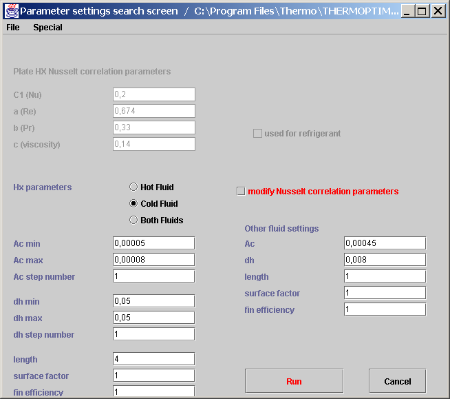
Figure 5.3.1: Heat exchanger screen setting
Moreover, are taken into account:
- the length of the exchanger (for the calculation of boiling number Bo in evaporation correlation);
- the surface factor;
- the fin efficiency.
Three options are possible for choosing the search of the optimum pair (Ac, dh) "Hot fluid" for the sole hot fluid, "Cold fluid" for the sole cold fluid, and "Both fluids" for both. In the latter case, identical values of parameters (Ac, dh, L, f and ηf) are set on both exchanger fluids (reasonable assumption for plate heat exchangers, a priori symmetrical). In other cases, parameter values appearing under "Other fluid settings" are set, constant, for the fluid not selected.
It is difficult to define an indicator of accuracy which gives full satisfaction, because the differences between model predictions and experimental data can be measured many ways, no one a priori knowing which is the best. In a heat exchanger, it seems natural to look for differences obtained on the fluid outlet temperatures, but on the one hand their off-design calculation can be relatively long, and secondly the weighting between them would affect the test. To accelerate calculations, we found it preferable to compare the values of the exchange surfaces predicted by the model in design mode.
The "Run" button is launching iterations during which the surface of the exchanger is determined in technological design mode for all project files placed in directory "param_search". Simulation results are stored in file "simul.txt" which can be opened in a spreadsheet. For the launch of iterations to be possible, file "simul.txt" must be closed.
Line "Simulate and save" of the "Special" menu allows to enable or disable the request by Thermoptim of simulated projects backup. In general, it is best to disable this function, so that this request is not made at each project loading, especially since the final setting corresponds to the highest bounds of the ranges of variation of Ac and dh. Once the optimum found, you can restart the process with a number of increments equal to 1 for both values to force the update of the parameters obtained. It is then possible, by clicking "Run" to save the various files in the directory "param_search", which allows to update them with the values found. Note that it is also possible to set these values using the project file change mechanism presented section 5.2.1.
Menu File offers two lines that allow to save the complete set of values in the screen in Figure 5.3.1 or reload them.
5.3.3 Exploitation of file simul.txt
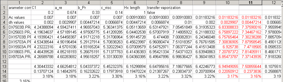
Figure 5.3.2: Simulation results
File "simul.txt" can be copied into a spreadsheet like the one in Figure 5.3.2.
Bottom lines of the worksheet allow to calculate the mean, standard deviation and an indicator of identification accuracy, which we call the exchange surface dispersion, equal to the ratio of standard deviation to the mean value. In the example given, minimum dispersion is 3.16%. The first lines of the file give the values chosen for correlation settings.
To find the most likely setting, it is necessary to try several and compare. Experience shows that better accuracy can be obtained with several values of the surface (in the example above, 6.15 m2 and 7.51 m2 are equivalent). An indication of the design value of the surface is therefore necessary to remove the doubt.
5.3.4 Identification method
To achieve good convergence of the identification process, we proceed as follows:
- we first choose for each the most relevant fluid flow pattern, and we estimate parameters Ac, dh, f, length... from geometric data. They are used to set the initial project file;
- we generate project files corresponding to the experimental data using the screens shown section 5.1;
- we test a first set of heat exchanger parameters with all available points, and we study the extreme values of the calculated results;
- on the basis of this review, we change the settings to reduce the gap (on a representative subset of the data if there are many), and parameters are optimized by reducing the dispersion regardless of the average surface value;
- we test the parameter set obtained on all points;
- finally, we seek to obtain the correct value of the exchange surface (corresponding to that given by the manufacturer), inspired by the approach described Section 5.3.5.
6 Productive structure editor
A new editor including the various components used in the productive structures has been developed (figure 6.1).
Figure 6.1: Productive structure editor
It is accessible from the "Special" menu of the simulator screen (Ctrl B). Its palette provides icons for process-points

to represent inlet and outlet flows, for PDUs

, and for junctions

and branches

.
This productive structure editor being analogous to the diagram editor, the details of its basic functionality is given in Volume 1 of Thermoptim reference manual.
A productive structure can be built either by hand by selecting the icons on the palette and connecting them, or automatically by deriving it from the physical diagram and from the simulator settings.

Figure 6.2 : productive or dissipative unit
6.1 Productive or dissipative units
The exergy resources being of three possible types, and the products of two, a productive unit is represented by a rectangle with three inlet ports and two outlet ones (figure 6.2), whose colors are differentiated in order to distinguish the various types of exergy flows and to allow to graphically separate resources and products.
The inlet port colors are the following: red for fuel, blue for mechanical power, and green for fluid exergy variation; the outlet port colors : blue for mechanical power, and green for fluid exergy variation.
The exergy flow values can be displayed on the links, which are colored similarly.
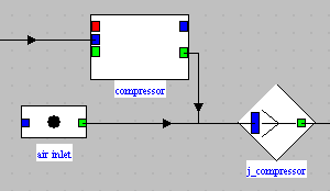
Figure 6.3: exergy provider
6.2 Junctions and branches
The exergy of a fluid going through a component can increase or decrease. If it increases, we shall say that the component is an exergy provider, if it decreases that it is an exergy receiver.
An exergy provider is represented by a productive unit with a junction at the outlet, with two incoming links: the one going out of the green port of the productive unit (outlet exergy flow), and the one corresponding to the inlet exergy flow (figure 6.3).
On this figure, the total exergy available at the outlet of the pseudo-node "j_compressor" is the sum of two values: first the exergy flow at the inlet of the component, represented by the process-point "air inlet", and second the exergy variation of the fluid in the compressor, which gets it under a mechanical form. The pseudo-mixer or junction "j_compressor" is used to model this addition.
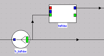
Figure 6.4: exergy receiver
An exergy receiver is represented by a productive unit with a branch at the inlet, with two outgoing links: the one arriving at the green port of the PDU (inlet exergy flow), and the one corresponding to the outlet exergy flow (figure 6.4).
On this figure, the total exergy available upstream of the turbine separates in two parts: first the one which is the turbine "fuel" and is converted under a mechanical form, and second the one which remains available at the turbine outlet. The pseudo-divider or branch "b_turbine" is used to model this division.
It should be noted that, for the provider components (those for which ∆Xh > 0), Pi = ∆Xh. For the turbine (for which ∆Xh < 0) Pi = τ. The throttlings being purely dissipative, Pi = 0.
6.3 Automatic generation of productive structures
It is possible to construct by hand with Thermoptim the productive structure of an energy system, but this is not the best way to operate if one knows the physical sketch, as is usually the case.

Figure 6.5: Main menus
The productive structure can very well be inferred from the physical sketch (Thermoptim diagram) and thermodynamic parameters (Thermoptim project). Provided that the temperature T0 of the surroundings is properly initialized (Help menu / global settings of the simulator), it serves to distinguish the exergy providers and reducers, and calculate exergy balances of PDUs.
In a first step, by selecting the line "Diagram transfer " of menu "Special", it creates all production units within the rules of correspondence stated above. It should be understood that a Thermoptim project and its diagram should have been previously opened and recalculated.
It should be noted that this way of doing may result in the introduction of junctions in series and/or of branches in series, which may be grouped in order to simplify the productive structure. This happens when several providers or several receivers appear sequentially in the physical diagram. This is for instance the case when a phase change heat exchanger such as a steam generator is represented by three exchangers in series (economizer, vaporizer, superheater).
It is therefore possible, in a second step, to select the pseudo-nodes in series the structure editor, and group them by selecting the line "Suppression of nodes in excess" of menu "Special". In order to avoid errors, you can choose not to automatically remove the real nodes appearing in the physical structure, knowing that they can be removed by hand in a second time.
At this stage, the blue exergy inlets (mechanical power) are not connected, or the temperatures of the external sources with which heat-exergy is exchanged are not entered. It is therefore necessary, in a third step, to set some additional parameters in the productive structure, in particular in the exergy balance screens presented below.
6.4 Component exergy balances
In Thermoptim, the logical link between the productive structure and the simulator is made by the component name. We must therefore call the UPD by the same name as the corresponding element of the simulator.
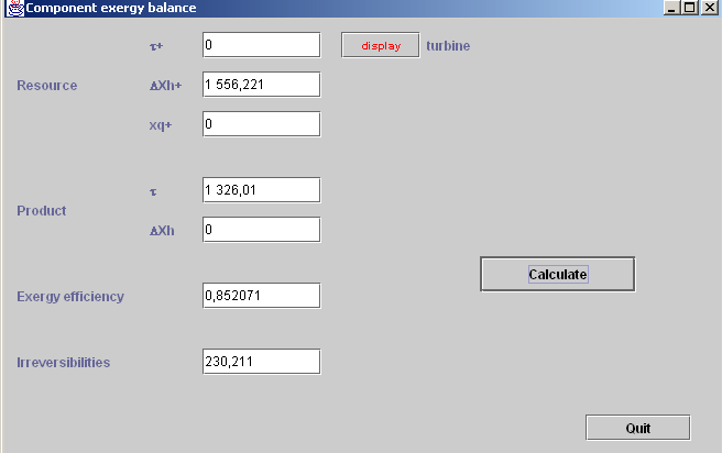
Figure 6.6: Exergy balance of a turbine
Double-clicking a productive unit allows one to open a component exergy balance screen, in which can be entered the settings which are required for calculating the exergy resources and products, as well as the component irreversibility and exergy efficiency (figures 6.6 et 6.7).
Figure 6.6 shows the screen of a turbine component: the exergy resource is provided by the fluid exergy variation (∆Xh+), the product is the mechanical power (τ+), and the exergy efficiency and irreversibilities are also determined.
When the component is of the exchange type, different possibilities exist.
If it is a fluid inlet or outlet, which corresponds in Thermoptim to a process-point connected only upstream or downstream, its exergy must be taken into account in the balance by determining its exergy contribution as compared to the reference conditions, i.e. its relative exergy.
If it is a fluid outlet rejected in the environment, the exergy is lost, which corresponds to an irreversibility. If on the contrary this exergy has an external value, it is an exergy product without irreversibility.
When internal heat exchanges occur, as for instance in combined cycles, the exergy loss calculation must also be modified: it is equal, in absolute terms, to the sum of the exergy variations of both fluids exchanging heat. The component exergy balance screen has an option (Internal exchange) for this setting (figure 6.7). We shall see later that, in the overall exergy balance, the exergy variations of both fluids are displayed between brackets.
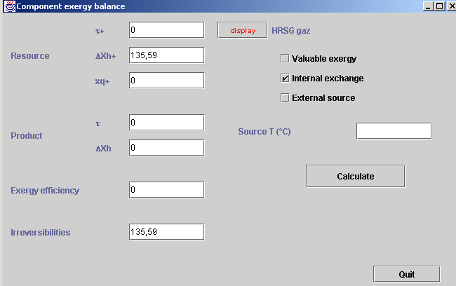
Figure 6.7: Exergy balance of an exchange process with internal exchange
Lastly, when the heat exchange takes place with an external energy source, the heat-exergy involved must be assessed, which requires the knowledge of the source temperature. This information may be entered in the exergy balance screen.
For throttlings, the input exergy is the inlet relative exergy, and the output exergy the outlet relative exergy. The irreversibility is equal to their difference.
As exergy providers are represented by a PDU coupled to a mixer, it is necessary to clearly distinguish these pseudo-mixers from the real ones which appear in the physical system, as the irreversibility in a real mixer may stem from different sources:
- reduction of a fluid pressure (pressure drop)
- mixing with composition change
Appendix 2 explains how the various types of components most generally used in energy systems (which are included in Thermoptim core) can be represented as PDUs.
External components can also be represented in a productive structure. Please refer to the Volume 3of the Reference Manual for details on this.
6.5 Generation of exergy balances
Once a productive structure is built, the exergy balances of the various components may be either calculated one by one in their respective screens, or globally for the whole project , by selecting the line "Project exergy balance" of menu "Special". Thermoptim then builds a table whose rows correspond to each component, plus one for the system as a whole. The latter gives as resource the sum of the positive heat-exergies and useful work provided , as product the sum of the of exergies leaving the system, the exergy efficiency of the system, and the sum of irreversibilities. If the rules for building exergy balance adopted in Thermoptim do not give satisfaction, the user can export it in order to modify it in a spreadsheet.
In a project exergy balance, the exergy variations of the fluids coupled by a heat exchanger are represented between brackets in the irreversibility column, the name of the exchanger being displayed on the right. The heat exchanger irreversibilities are equal to the algebraic sum of the values between brackets for both fluids involved (figure 6.8).
Examples of productive structures and corresponding exergy balances for a steam power plant, a refrigeration machine and a cogeneration gas turbine are given in Chapter 10 (Part 3) of the book Energy systems.
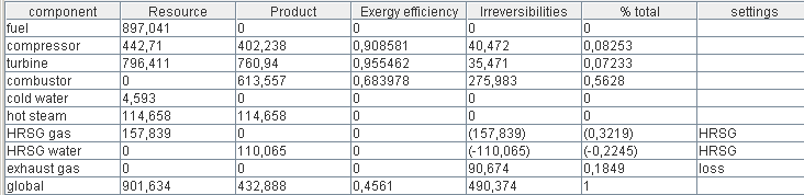
Figure 6.8 : Exergy balance of a cogeneration gas turbine
Appendix 1: classes ExtPilot, PointThopt, CorpsThopt
In this appendix, we give some indications on the three classes ExtPilot, PointThopt and CorpsThopt that have been defined to facilitate the creation of advanced external classes, including drivers.
Class ExtPilot
This is the superclass of all drivers. To secure the setting of the different methods allowing to update the core Thermoptim objects it offers, it defines a number of directly understandable booleans:
boolean RECALCULATE=true, UPDATE_T=true, UPDATE_P=true, UPDATE_X=true, UPDATE_ETA=true, UPDATE_UA=true, UPDATE_EPSI=true, UPDATE_FLOW=true, IS_SET_FLOW=true, UPDATE_DTMIN=true;
In this way, the following code updating a point:
avalFroid.update(UPDATE_T,!UPDATE_P,!UPDATE_X);
reads as only update the avalFroid point temperature, which is much more readable than :
avalFroid.update(true, false , false);
public void updateprocess(String name, String type, boolean recalculate, boolean isSetFlow, boolean updateFlow, double flow,
boolean updateParam1, double param1, boolean updateParam2, double param2)
Available with several signatures, this method updates and recalculates a process. If recalculate is true, it is recalculated, if isSetFlow if true, its flow is set, if updateFlow is true, its flow is set to flow, if updateParam is true, the parameter value is set. The meaning of arg depends on the type and can be solved by referring to the Project method updateProcess(), as defined in Volume 3 Reference Manual.
For example, the following code updates the process name compressorName, of the Compression type, request the recalculation, sets the flow rate by changing its value, and modifies the isentropic efficiency:
updateprocess(compressorName, "Compression",RECALCULATE,IS_SET_FLOW, UPDATE_FLOW, massFlow, UPDATE_ETA, eta_is);
Similarly, methods for updating and recalculating for heat exchangers and nodes exist:
public void updateHx(String name, boolean recalculate, boolean updateUA, double UA,
boolean updateEpsi, double epsi, boolean updateDTmin, double DTmin)
public void updateNode(String name, boolean recalculate, boolean updateEffectiveness, double epsi)
Both methods transferTechnoData () and setupTechnoDesigns () are used to initialize the driver and technological screen while opening an existing project file.
The first method includes all lines in project file on technological screens and loads them in the driver when it is built, and the second decodes these lines to perform its initialization, calling the standard TechnoExch methods, which call on FlowConfig.
The last setupTechnoDesigns()line proj.bindTechnoDesigns(vSettings), is used to link the TechnoDesign used by the driver with the core components, so they can be displayed from their screens and global tables of the technological and simulation screen.
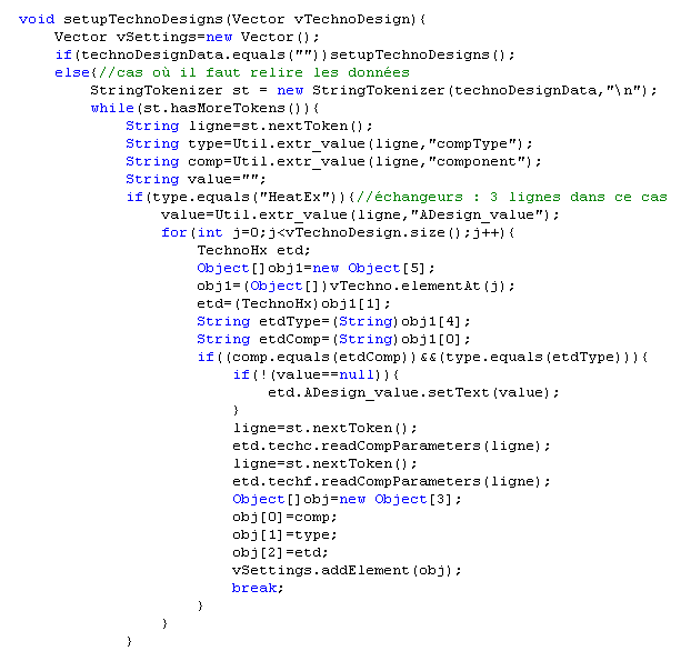
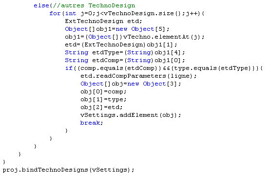
Class PointThopt
This class creates kinds of external clones of core Thermoptim points, in order to have easy access to their values, which are not otherwise directly accessible. It provides more comfort and clarity than does the use of Project methods getProperties() and updatePoint(), documented in Volume 3 Reference Manual. It includes double values that store equivalents of core state variables:
double W,Epsi,QPrime,Tprime,Tr,VPrime,Cond, M_sec, corrFactor;
CorpsThopt corps;
During construction, it specifies the reference to the project and the name of the point in the simulator, which allows Thermoptim to know which point is concerned. Caution, if an error occurs at this level, the PointThopt cannot be properly instantiated.
public PointThopt(Projet proj, String name){
this.proj=proj;
this.name=name;
try{
getProperties();
}
catch(Exception e){
String msg = "Error constructing the PointCorps name: "+ name;
JOptionPane.showMessageDialog(new JFrame(), msg);
e.printStackTrace();
}
corps=new CorpsThopt(proj, nomCorps,lecorps);
}
PointThopt also offers methods to update its simulator equivalent, based on the same principle as those of ExtPilot with signatures depending on the number of values to change.
public void update(boolean updateT, boolean updateP, boolean updateX, boolean updateCorrFactor, boolean melHum, String task, double value)
A most common lighter version served as an example explaining the use of explicit ExtPilot booleans:
public void update(boolean updateT, boolean updateP, boolean updateX){
update(updateT, updateP, updateX, false, false, "", 0.);
}
Class CorpsThopt
This class creates kinds of clones of core Thermoptim substances, to have easy access to their values, which are not otherwise directly accessible. It provides more comfort and clarity than does the use of Project methods getProperties() and updateSubstance(), documented in Volume 3 Reference Manual. It has double variables that store the equivalent of the core state variables:
public double T,P,X,V,U,H,S,M,M_sec,TC,PC,VC;
During construction, it specifies the reference to the project and the name of the substance in the simulator, which allows Thermoptim to know which substance is concerned. Caution, if an error at this level, the CorpsThopt cannot be properly instantiated.
public CorpsThopt(Projet proj, String name, Corps lecorps){
this.proj=proj;
this.name=name;
this.lecorps=lecorps;
}
An instantiation example is given in the PointThopt constructor.
Mmethod getSubstProperties() allows to update the values after a calculation on variable lecorps. The example below shows using a CorpsThopt using PointThopt "amont":
CorpsThopt corps=new CorpsThopt(proj,amont.nomCorps, amont.lecorps);
corps.lecorps.CalcPropCorps(amont.T,amont.P,1.);
corps.getSubstProperties();
Usual functions are then directly accessible: for example, enthalpy is given by corps.H.
Classes for technological design
The classes for compressors and exchangers have been presented Section 3.2. Let us recall that these classes should be considered only as templates intended to be refined by users who wish to study the technological design and off-design behavior of systems, and not as well validated models. Our goal is simply to facilitate their efforts by providing them with practical examples on which they can elaborate.
To introduce new classes, just subclass existing ones, or create new ones based on the same model and place them in extThopt.zip or extUser.zip for version 1.7 and extThopt2.zip or extUser2.zip for version 2.7.
Classes for turbines
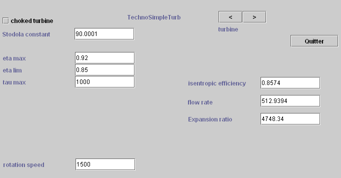
Figure A.1 : Basic simple-stage turbine technological design screen
Modeling turbine off-design operation is a problem that can be addressed with varying levels of difficulty. Therefore we implemented a series of different models, to graduate the approach depending on the available data and the the user level:
The basic class is TechnoSimpleTurb. It is based on the rule of the cone and strictly speaking only applies to a single-stage turbine:
- Class TechnoMultiStageTurb extends the previous one considering that the rule of the cone of the multi-stage turbine is the same as that of a single-stage turbine, the expansion ratio to take into account being the nth root of the total expansion ratio if n is the number of stages. If n = 1, the behavior is the same as that of the previous class;
- Class TechnoTurb extends the previous one, allowing to take into account both the existence of residual velocity losses (RVL) at the turbine outlet, and also a deterioration in isentropic efficiency in the wet zone following the Baumann rule;
- Class MultiStageMappedTurbine extends the previous one, the rule of the cone being this time replaced by a mapping represented by a numerical adjustment to twenty parameters.
TechnoSimpleTurb
This class defines the technological design parameters for turbines (figure A.1).
The meaning of the fields is as follows:
- Stodola constant is the Stodola coefficient. If "choked turbine" is checked, the flow is regarded as shocking, and the formula used is (A.1). Otherwise, it is (A.2);
- where η is represented by an 3 parameter equation, eta max is the maximum value, eta lim the limit for the very high expansion rates, and tau max the abscissaof the maximum. If the first two values are equal, the isentropic efficiency is constant;
- rotationspeed is the speed of rotation ;
TechnoMultiStageTurb
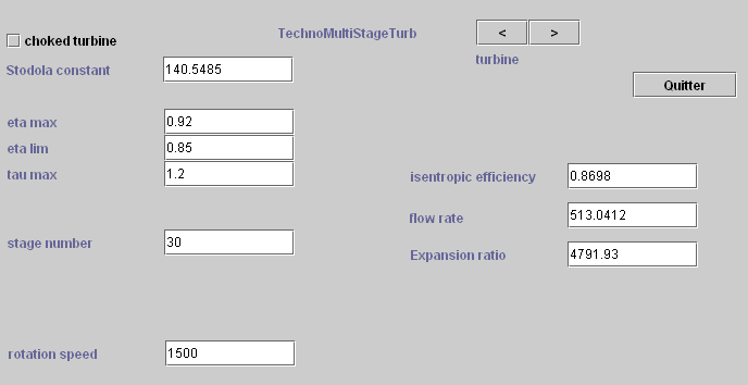
Figure A.2 : Multi-stage turbine technological design screen
The difference between its screen and the preceding is the introduction of a new field, representing the number of turbine stages (figure A2).
Stodola's formula taken into account is more general than (A2), and takes into account the polytropic coefficient of expansion.
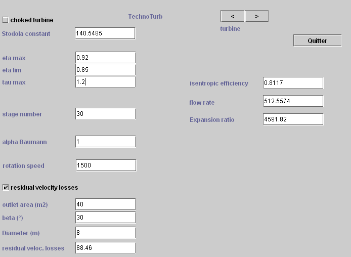
Figure A.3 : Multi-stage turbine technological design screen
TechnoTurb
Its screen (Figure A3) differs from the preceding by the several new fields. As mentioned above it takes into account the existence of residual velocity losses (RVL) at the turbine outlet, and a reduction of the isentropic efficiency in the wet zone, according to the Baumann rule (A3).
The values of residual velocity losses appear on the left of the screen.
ηhum = ηdry (1 - α (1 - x)) (A.3)
The meaning of the fields is as follows:
- alpha Baumann is the coefficient α of equation (A.3);
- for calculating residual velocity losses, it is necessary to provide the outlet section and the diameter of the turbine, as well as the output angle β.
Class MultiStageMappedTurbine
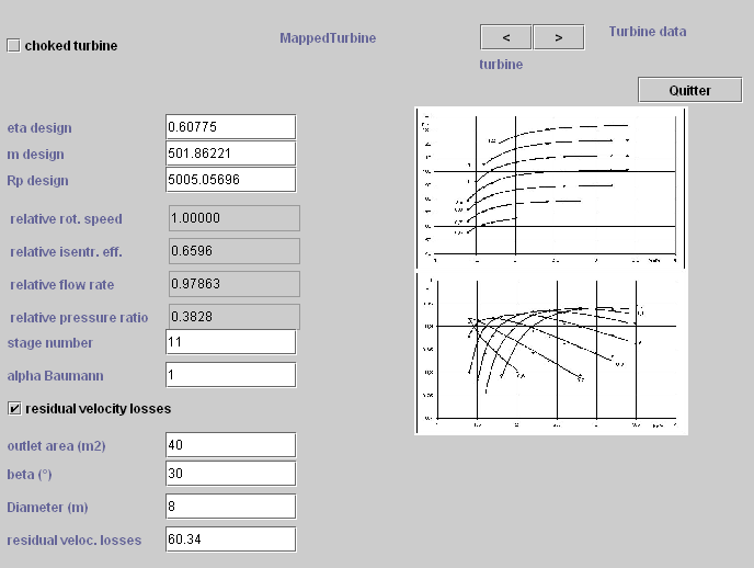
Figure A.4 : Turbine technological design screen with mapping
This class, which inherits from TechnoTurb defines the technological design parameters for turbines represented by detailed mapping, as defined in a modeling note.
The technological screen (figure A.4) has in its upper right a label ("Turbine data") which provides access by double-clicking to the screen displaying the series of coefficients describing flow rate and isentropic efficiency characteristics (class TurbineMapDataFrame, figure A.5).
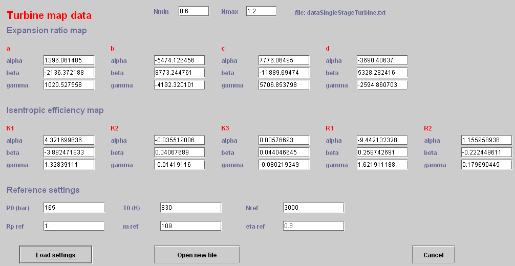
Figure A.5 : Turbine mapping setting screen
To the right of figure A.4 appears inset image corresponding to selected characteristics, if loaded. Otherwise the label "Turbine maps" allows to open by double click an image loading screen (class MapImage).
The data files and images of maps must be placed in the "maps" directory from which both classes work. Their names must be saved by the driver.
The mapping used here is expressed on a normalized flow. During design, we hold the nominal point of the mapping on that the expansion process (later, we should be able to deduce the size, but this not yet implemented), which provides the values "eta design","Rp design"and"m design"displayed in the left of the screen.
Below them appear dimensionless values needed to set the operating point on the mapping used. Their values are of course adjusted to the turbine inlet conditions.
The value of the rotation speed can be set from the driver screen if desired.
Class TechnoNozzle
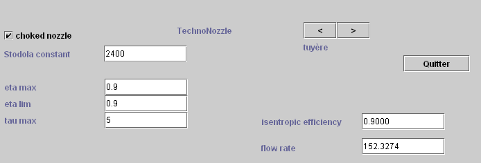
Figure A.6 : Design screen for a nozzle
This class defines the technological design parameters for nozzles (figure A.6).
In off-design operation, a nozzle can be modeled similarly to a turbine, and characterized by a Stodola constant and an isentropic efficiency. Its screen corresponds to the upper part of that of the simple-stage turbine.
Class TechnoTurboCompr
This class defines the technological design parameters for turbocompressors.
The technological screen (figure A.7) uses a series of coefficients describing both characteristics.
Corrected reduced flow in the compressor:
Reduced compressor characteristic:
ψ = ψcoeff (A.5)
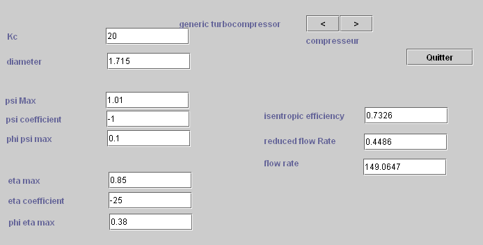
Figure A.7 : Turbocompressor technological design screen
The parameters to define are the following:
- Kc, compressor characteristic (equation (A.4));
- the compressor diameter;
- ψ is represented by a branch of a parabola, defined (equation (A.5)) by ψmax, maximum value, ψcoeff and ϕψmax, abscissa of the maximum corrected flow mc;
- η is also represented by a branch of a parabola, defined by ηmax, maximum value, ηcoeff and ϕηmax, abscissa of the maximum corrected flow mc.
The values of isentropic efficiency, flow and reduced mass flow appear on the right of the screen.
Class MultiStageMappedTurboCompr
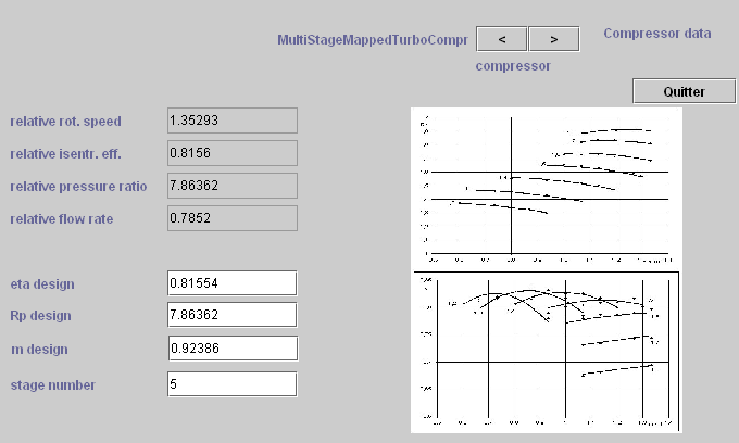
Figure A.8 : Design screen of a turbocompressor with mapping
This class, which inherits from TechnoTurboCompr defines the technological design parameters for turbocompressors represented by detailed mapping, as defined in the modeling note quoted above.
The technological screen (figure A.8) has in its upper right a label ("Compressor Data") which provides access by double-clicking to the screen displaying the series of coefficients describing flow rate and isentropic efficiency characteristics (class TurboComprMapDataFrame, figure A.9).
To the right of the figure A.9 appears inset image corresponding to selected characteristics, if loaded. Otherwise the label "Compressor data" allows to open by double click an image loading screen (class MapImage).
The data files and images of maps must be placed in the "maps" directory from which both classes work. Their names must be saved by the driver.
The mapping used here is expressed on a normalized flow. You must enter in the data file all reference values: P0, T0, Nref, Rpref, mref, etais_ref, as well as the interval of variation of the reduced speed (here 1.2 to 1.8).
During design, we hold the nominal point of the mapping on that the compression process (later, we should be able to deduce the size, but this not yet implemented), which provides the compression rotation speed and values "eta design","Rp design"and"m design"displayed in the left of the screen, and potentially modifiable.
Above them appear dimensionless values needed to set the operating point on the mapping used. Their values are of course adjusted to the compressor inlet conditions.
Below these values is the field for defining the number of steps if you use a generic mapping (here 5).
The value of the rotation speed can be set from the driver screen if desired.
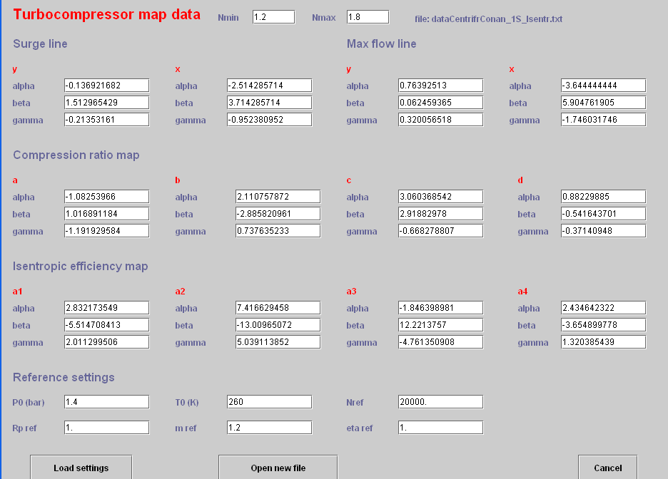
Figure A.9 : Screen defining parameters of mapping of turbocompressor
Remarks on the reference values of mapping files
The last lines of file mapping (bottom screen figures A.5 and A.9), provide the benchmarks that allow mapping to adapt to a given problem. The pressure and inlet temperature and speed of rotation generally correspond to those of the simulator for the nominal point. The ratio of compression / expansion and isentropic efficiency / polytropic should be equal to 1 if the mapping corresponds to the compressor used, but they can be modified if necessary. The value of the reference flow will typically close to the speed of compressor nominal point, since the maps were prepared for flow rates normalized.
Appendix 2 : Representation of simple components as productive units
Exergy provider components
Combustion: F = P =∆xh
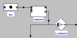
A combustion chamber converts the fuel exergy xq+ (represented by a link arriving in the red port) in an exergy increase ∆xh of the fluid. A junction must therefore be placed downstream; its other inputs are for instance the oxidizer and the compressor. The outgoing link comes from the green port.
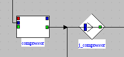
Compressor with internal exergy input: F = P =∆xh
A compressor (or a pump) converts the mechanical power τ+ received in an exergy increase ∆xh of the fluid. A junction must therefore be placed; its other inputs are for instance the oxidizer and the combustion chamber. The outgoing link comes from the green port.
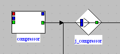
Compressor with external exergy input: F = P =∆xh
If the power received is internal, it is represented by a link entering the blue port. If it is external, it is not displayed on the editor, but is taken into account in the exergy balance screen.
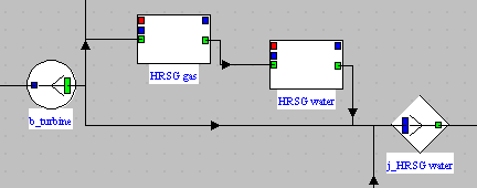
Internal heat exchange hot fluid upstream, cold fluid downstream: F = P =∆xh
In a heat exchanger modeled as the coupling of two exchange processes, the resource corresponds to the exergy variation of the hot fluid, and the product to that of the cold fluid. The hot fluid must therefore correspond to one of the branches of a divider, and the cold fluid to one of the branches of a junction. Both components are connected as shown on figure.
External heat exchange Q>0

F = P =∆xh
In a heat exchange with an external source with a temperature greater than that of the environment, bringing heat to the system, the resource is the heat-exergy xq+ transferred from the source. This heat-exergy is converted en accroissement in an exergy increase ∆xh of the fluid. A junction must therefore be placed downstream. The outgoing link comes from the green port.
Exergy receiver components
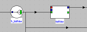
Turbine: F = P =
A turbine converts in mechanical power τ the exergy decrease ∆xh+ of the fluid (represented by a link entering the green port). A branch must therefore be placed upstream; it must at least have another output, such as the exhaust gases rejected in the atmosphere, or a condenser if steam is being expanded. The outgoing link comes from the blue port.
External heat exchange Q<0
Tk > T0
F =
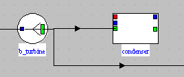
When the system is cooled by an external source whose temperature is greater than that of the environment, the heat-exergy lost is equal to the exergy decrease ∆xh+ of the fluid (represented by a link entering the green port). A branch must therefore be placed upstream; it must at least have another output. The temperature of the external source must be entered in the PDU exergy balance screen.
External heat exchange Q>0
Tk < T0
F =
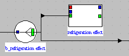
When the system is heated by an external source whose temperature is lower than that of the environment, the heat-exergy lost xq- is equal to the exergy decrease ∆xh+ of the fluid (represented by a link entering the green port). A branch must therefore be placed upstream; it must at least have another output. The temperature of the external source must be entered in the PDU exergy balance screen.
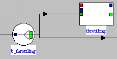
Throttling F = P = 0
In a throttling, the relative exergy of the fluid decreases between the inlet and the outlet of the du component, because of the pressure drop at constant enthalpy. A branch must therefore be placed upstream. This component is purely dissipative.