Thermoptim reference manual Volume 2
Table of contents
Copyright © R. GICQUEL 1997-2022 All rights reserved. This document may not be reproduced in whole nor in part without the author’s express written permission, except for the personal licensee’s use and solely in accordance with the contractual terms indicated in the software license agreement.
Information in this document is subject to change without notice and does not represent a commitment on the part of the author
Foreword
Thermoptim documentation
Thermoptim documentation is comprised of several complementary parts:
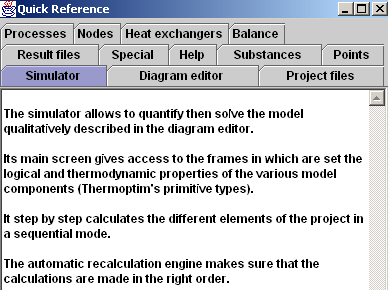
- a short documentation named Quick Reference available through menu Help: it gives access to tab frames introducing the main concepts used
- a printable documentation, mainly as pdf files
- on line e-learning modules with sound tracks named Diapason
- guided explorations of Thermoptim models
Printable documentation
The printable documentation is comprised of several parts which can be displayed through the Help menu of the simulator:
- Four Getting Started brochures allow one to quickly (less than half an hour) get used to Thermoptim. The first one presents an electricity steam cycle, the second one a combustion gas turbine, the third one a refrigeration cycle and the fourth one an air conditioning system
- The reference manual, itself comprised of three volumes and of the interactive charts manuals. The first volume introduces the software, the diagram editor, the use of the post-processing Excel macro and the optimization method, the second one deals with the simulator (screens of the different primitive types and advanced tools available in the modeling environment), and lastly the third volume explains how to use and build external classes
- a Frequently Asked Questions file is also available
Several examples with detailed explanations allow a user to get acquainted with the software thanks to a detailed presentation of how projects can be built. Three of the examples extend the Getting Started brochures.
The present document is the first volume of the reference manual. After a short introduction of the software, it presents the diagram editor and the optimization method.
Access the documentation via hypertext links
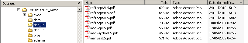
Windows versions 1.5 and later include hypertext links that provide direct access to the documentation and the FAQ. In order for the links to work, the file paths must be identical to what was entered in Thermoptim, otherwise they will not appear on the list.
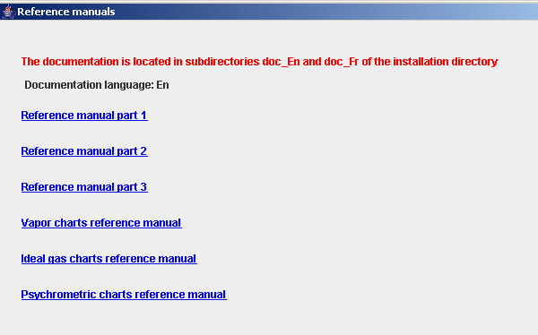
The documentation in English must therefore be structured as shown in the figure below. If you have an older installer, rename the files accordingly.
Diapason, online e-learning modules with audio
We have developed DIAPASON e-learning modules, which are online instructional modules with audio and animation allowing users to work on their own, at their own pace, with access at all times to oral explanations in addition to the written materials provided.
The following session is dedicated to being introduced to Thermoptim (in English):
https://direns.mines-paristech.fr/Sites/Thopt/en/co/session-s07en_init-first.html
There is also a special unit specifically on how to use and program external classes (in English):
https://direns.mines-paristech.fr/Sites/Thopt/en/co/session-s07en-ext.html
The purpose of these sessions is to introduce users to Thermoptim and enable them to become familiar with using it by building models using examples of simple energy systems (gas turbine, steam power plant, compression refrigeration system).
Guided explorations
In guided explorations of models built with Thermoptim, learners explore and parameterize models already built.
In Diapason sessions, learners learn how to build models on their own.
In , to reduce the difficulties associated with using the software package, they explore and parameterize models already built.
These guided explorations offer different activities to learners, such as finding values in the simulator's screens, resetting it to perform sensitivity analyses... Contextual explanations are given to them gradually.
Demonstration versions
All functions presented in the reference manual are not available in Thermoptim demonstration versions 2.5 and 2.82. In these versions the number of points and processes is limited to 10, the chart interactivity is disabled, as well as the advanced tools for diagnosis, automatic recalculation (including pressure settings), sensitivity studies and optimization. Furthermore only a subset of substances is available and all saving functions are disabled. It is however possible to read any Thermoptim project (whatever its size).
Version 2.82 is the one used in directed explorations.
The demo versions can be downloaded from this page.
Basic notions
The study of a thermodynamic system can be divided into five main tasks:
- 1) the analysis of the structure of the system under investigation, which identifies its main components and their connections: for instance, a thermal machine consists of heat exchangers, compressors, turbines or expansion devices, combustion chambers...
- 2) For each component, the identification of the thermodynamic fluids which are used: for instance, the fluid compressed in a gas turbine is air, which burns with a fuel in the combustion. The resulting flue gases expand in a turbine.
- 3) for each component, the selection of the kind of system to be considered (open or closed): for instance, the study of the compression in a piston compressor must be made in closed system, while that of the expansion in a gas turbine is to be made in open system.
Let us recall that a closed system (respectively an open system) is characterized by the absence (respectively the existence) of mass transfer through its boundaries.
- 4) The description of the processes which undergo the different fluids in the components, and the calculation of their evolutions in the components, taking into account their interconnections.
- 5) The calculation of the overall balance of the system analyzed.
THERMOPTIM focuses on the global behavior of thermodynamical systems, considering that the detailed internal design of components requires specific tools taking into account all sides of the problem (scientific bases, but also manufacturing and economical constraints). Fortunately, it is not necessary to have access to the detailed internal behavior of a component in order to be able to study how it fits inside a system. Generally, and this is true for most energy technologies, a component can be characterized by a small number of parameters and the values of its coupling variables. These parameters vary according to the type of component: a volumetric compressor is characterized by a volumetric compression ratio, a volumetric efficiency and an isentropic efficiency, a heat exchanger by an effectiveness and a number of transfer units… Coupling variables are pressures, temperatures, flow-rates…
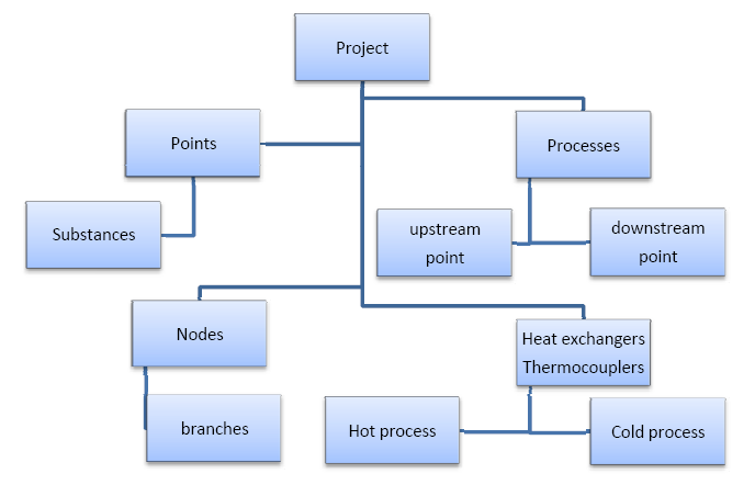
The list of the main different functional elements which may be used for describing a thermodynamical system strictly corresponds to the concepts which are used in THERMOPTIM. We shall refer to it later as its set of primitive types. It includes the thermodynamic fluid properties, the points, the processes, the nodes and the heat exchangers described below, which are always grouped in a project.
THERMOPTIM has been designed in order to facilitate the calculation of complex thermodynamic systems, but it cannot replace the user for making the detailed analysis of the system under investigation, which corresponds to the three first steps above. Before entering his project in the software, the user must have made this analysis. Otherwise there is a risk that the description will be done improperly.
In this regard, the primitive type set used in THERMOPTIM constitutes a useful guide for modeling the system under consideration, and the software provides the user with analytical tools which allow him to check the interconnections by navigating between the different elements of the project.
Thermodynamic properties of substances
THERMOPTIM makes use of three kinds of substances: pure ideal gases, compound ideal gases and condensable vapors (which are pure substances). Perfect gases are ideal gases whose specific heat is independent of the temperature. A given substance may exist (under different names) as an ideal gas and a condensable vapor.
The substance can be pure, in which case its properties are predefined in the software, or it can be compound. In this case (that is possible only for a gas), the user has to define the composition from the other gases present in the database, by indicating for each of them, its name and its molar or mass fraction. Properties of the composed substance are then determined from those of its constituents.
A particular substance exists in the database: it is called «generic liquid» (see below). It is a liquid at atmospheric pressure, whose specific heat is equal to 1 kJ/kg/K. It can be used to simulate any liquid not included in THERMOPTIM that one wants to use in a heat exchanger. However, the best way to introduce liquids is certainly to define external substances that Thermoptim is able to integrate into its database (see Volumes 1 and 3).
Data accuracy
Notice: the orders of magnitude of the accuracy given below are only illustrative and have no contractual value.
The thermodynamic properties of the ideal gases are calculated by regression from the data of the JANAF Tables [CHASE et al., 1985] using a 7 term polynomial equation. The state equation for all condensable vapors is a variant of that of Peng Robinson, except for water, for which were chosen the equations selected by the International Formulation Committee of the Sixth Conference on Steam Properties in 1967 [GRIGULL and SCHMIDT, 1982], which make use of a large number of parameters but are very accurate.
The accuracy of the calculations is excellent for ideal gases (error on the specific heat lower than 0.5 %), and for water (comparative tests with ASME steam tables give, for compressions and expansions, relative errors with enthalpies lower than 0.02 % in the vapor and liquid-vapor equilibrium, and lower than 0.5 % for the compressions in the liquid state).
For the other condensable vapors, the accuracy is slightly lower, the major deviations taking place in the liquid zone for reduced pressures greater than 0.7 and in particular supercritical. For these substances, liquid values are not modeled very accurately, the liquid being considered to be non compressible. In practice however, this is not very important for most applied thermodynamics processes.
Substance references
CHASE et al., Janaf Thermochemical Tables, J. Phys. Chem. Ref. Data, Vol 14 Suppl. 1, 1985
REID R. C., PRAUSNITZ J. M., POLING B. E., The Properties of Gases and Liquids, 4th Edition, Mc Graw Hill, 1987
GRIGULL U., SCHMIDT E., Properties of Water and Steam in SI units 0-800 °C, 0-1000 bar, 3rd Ed., Springer-Verlag, Berlin Heidelberg, R. Oldenbourg, München, 1982
DAUBERT T. E., DANNER R. P., SIBUL H. M., STEBBINS C. C., Physical and Thermodynamic Properties of Pure Chemicals : Data Compilation, Design Institute for Physical Property Data, ASME, Taylor & Francis, Washington, 1989-1997
Points
A point designates a particle of a substance and allows the user to define intensive state variables: pressure, temperature, specific heat, enthalpy, entropy, internal energy, exergy, and quality. A point is identified by its name and the name of the associated substance. To calculate it, one may either:
- enter the values of at least two state variables, generally its pressure and temperature for open systems, and its volume and temperature for closed systems.
- automatically calculate them by using for instance one of the processes defined below.
Processes
Processes correspond to thermodynamic evolutions undergone by a substance between two states. A process associates therefore two points such as defined previously, an inlet and an outlet point. Moreover, it indicates the mass flow rate involved, and allows one therefore to calculate extensive state variables, and notably to determine the variation of energy involved in the course of the process.
Processes can be of several types: compression, expansion, combustion, throttling, heat exchange, and water vapor / gas mixtures (the latter includes seven different categories of evolutions). According to each case, various characteristics of the process have to be specified, for example, in compression, its isentropic or polytropic efficiency.
As a point does not allow specification of the flow rate involved, it may be necessary to create particular processes, called processes-points, if needed. A process-point connects a point with itself, and indicates the mass flow rate required. Most of the time its type will be called «exchange».
A cycle can thus be described as a set of points connected by processes. To the extent that the mass flow rate fluid is the same in all the evolutions, processes and points are sufficient. If this is not the case, it may be necessary to describe at least partially the network of involved fluids. Then the first elements to define are the network nodes.
Nodes
Nodes allow one to describe elements of the system where mixes and divisions of fluids take place. In a node, several junctions of fluid are connected to form a single vein.
If the node is a mixer, the various branches join to form a single vein. The mass flow rate of the main vein is equal to the sum of these of branches, and the enthalpy balance allows one to calculate the mass enthalpy and the temperature of the mixture.
If the node is a divider, the main vein divides into several branches, whose flow must of course be calculated. Its distribution between the branches is set proportional to the "flow-rate factors" specified by the user. The temperature and the mass enthalpy are of course conserved. The separator is a special divider which separates the liquid and vapor phases of fluid in the liquid vapor zone.
One can mix several different fluids, provided that the mix is a gas. That means that if there are condensable vapors in the branches, one must make the hypothesis that they are in the gaseous state, and follow ideal gas behavior (this is why some substances exist at the same time as ideal gases and condensable vapors). Properties of the mix are calculated by application of the Dalton’s Law. The user has to verify that this hypothesis is valid. If this is not the case, results found by the software can be dissatisfactory.
The logical definition of a node is made by the association of processes, a process corresponding to the main vein (inlet process for a divider, outlet for a mixer), and n processes corresponding to branches. As the processes connect points, and each of these is linked to a substance, updates of flow rates and fluid states are made automatically by THERMOPTIM.
Heat exchangers
Thermal heat exchangers (or modules) connect two fluids, one that gets hotter, and the other that gets colder. The simplest definition for a heat exchanger can be made with the identification of the two processes (fluids) that meet. The design of the heat exchanger (presented in detail in Para. 2.10.3) can then be made if one indicates what constraints are set on the flow rates and temperatures (for instance minimum pinch, set value effectiveness).
Main project screen (simulator)
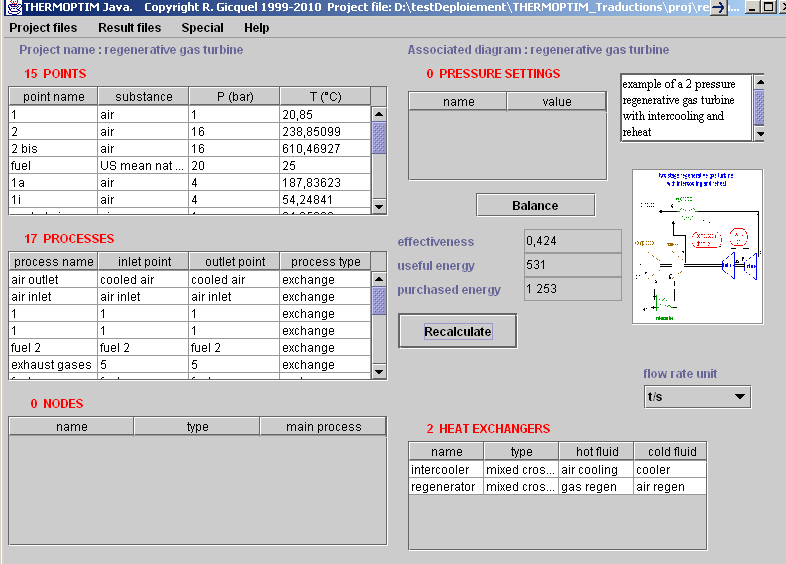
To get access to the different type screens, double-click either in the headband (creation of a new type) or on an existing line (for opening it). The text field in the upper right part of the screen allows one to enter a description of the project which can subsequently be used as a short summary. This description is displayed in the project library tables in order to enable the user to easily browse through his projects.
In the right part the button labeled "Balance" allows to calculate the overall balance with the following conventions:
In each process, the energy type allows one to distinguish between purchased energy, useful energy, and other energy (set by default). The purchased energy represents the sum of all the energies that must be supplied to the cycle from outside. The useful energy is the net energy output of the cycle, e.g. the algebraic sum of the energies internally produced and spent.
These two energy types are those that appear in the definition of the cycle effectiveness:
For example, in a Rankine cycle, the purchased energy is the heat supplied to the boiler and the useful energy is the net work output, i.e. the work output of the turbine minus the work input of the pump. The other energy is that used by the condenser. For a refrigeration cycle, the purchased energy is the input power of the compressor, the useful energy is the refrigeration effect (heat removed at the evaporator level), and the other energy is that removed at the desuperheater and condenser levels.
Just below, the button labeled "Recalculate" allows one to start the recalculation process, the number of invalidated and calculable elements being displayed.
In the right part of the screen appears a thumbnail of a block diagram representing the project studied if an image has been associated to it, or an empty frame otherwise. If you double-click in the frame, a window allowing to load or suppress the block diagram is opened.
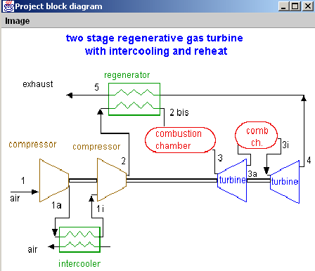
The menu allows you to open a .gif or .jpg image whose name is then saved in the project file. The image file has to be put in the same directory as the project to be automatically loaded with the project.
Main Menus
Menu "Project files" gives access to the following tools:
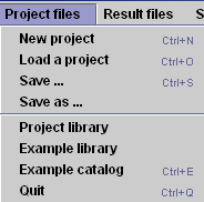
- "New project" creates a new project
- "Load a project" opens a project file and loads the project
- "Save …" saves the current project in the text file it was loaded from or it has been previously saved to. If the project is new, it must initially be saved by "Save as …", so that Thermoptim knows the file location and name
- "Save as …" saves the current project in the file you choose from a file dialog
- "Rename the project" enables you to rename the current project
- "Project library" opens a frame listing information on all project files in the user directory
- "Example library" opens a frame listing information on all example project files
Menu "Result files" gives access to the following tools:
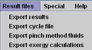
- "Export results" creates a text file in which detailed results of the project are saved
- "Export cycle file" creates a text file which can be read by the Interactive Vapor Charts for plotting the project points
- "Export pinch method fluids" creates a text file with the pinch method fluids which can be read by 4D Thermoptim version
- "Export exergy calculations" …..
Menu "Special" gives access to the following tools:
- "Diagram editor" allows one to graphically design a project
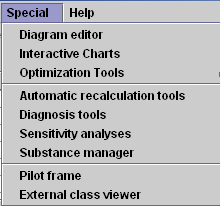
- "Interactive Charts" opens a frame allowing the user to display the project points in one of the three types of interactive thermodynamic charts (for vapors, ideal gases or psychrometric) and to create project points from these diagrams (see section "Interactive Charts" below)
- " Optimization Tools" opens the optimization frame (see section "Optimization tools" below)
- "Automatic recalculation tools" has been introduced above
- "Diagnosis tools" allow one to check a model's consistency
- "Sensitivity analyses" allow one to perform sensitivity studies on the current project
- "Substance manager"….
- "Pilot frame"…
- "External class viewer"…
Menu "Help" gives access to the following tools:
- "Reference manuals"…"Quick Reference" opens a frame giving the basic information on Thermoptim concepts and menus (see section "Quick Reference" below)
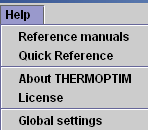
- "About THERMOPTIM" gives information on Thermoptim
- "License"….
- "Global settings" allows one to set the temperature unit, working directory...
Substance Manager
However, there is a problem with the substance names. In order to avoid generating errors, Thermoptim automatically constructs a compound gas whose default composition is either air or nitrogen when the user enters a substance name that is not in the database. When a file generated in French is read in English, the substance “water” will therefore be constructed as a compound gas. Clearly, this can be a problem, but there is no way to automatically translate substance names correctly, regardless of the language.
The solution is to use a tool that easily checks the way that the substances are instantiated and renames them. This tool is called the Substance Manager, accessible from the Special menu of the simulator. It enables the user to replace the substances of a project created in another language, or replace a substance throughout the project to test the influence of a substance change (for example, how changing the refrigerant stream affects the performance of a refrigeration cycle). This tool is not available in the demo version.
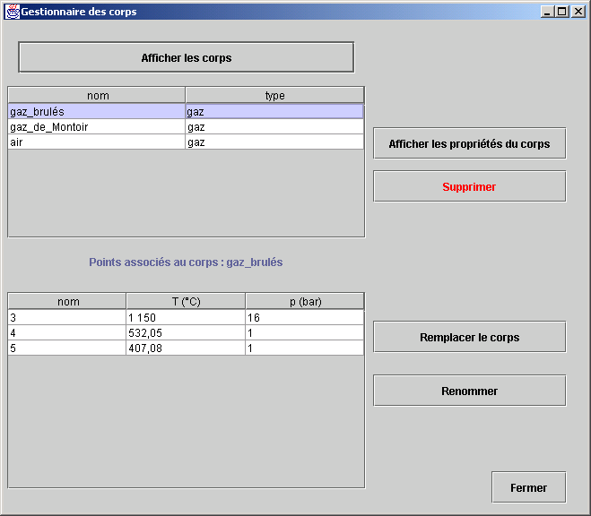
Clicking on “Display substances” located on the upper left displays a table of all the substances used in the project. If you click on one of the lines, the points linked to this substance are displayed in the table below. If a substance is not linked to any point, it can be deleted. If a line is selected and you click on “Display substance properties”, its composition is displayed if it is a gas, and its typical parameters are displayed if it is a vapor.
If you click on “Replace the substance”, the substance selection list is displayed so you can select the substance you want to use as a replacement. If you select one and click “OK”, all of the points linked to the first substance are modified accordingly and recalculated. Likewise, you can rename a substance provided that it is not a vapor. Obviously, the new name must not be the name of a pure or protected gas or a vapor.
Export of the results in the form of text file
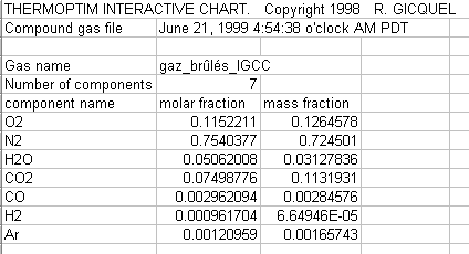
All the results corresponding to a project can be gathered in a text file which can be processed either by a word processor or by a spreadsheet. For that, select line "Export the results" of menu "Result files". A Save window is open so that you choose the backup file. Once that it is created, open it with a spreadsheet. You obtain the result below.
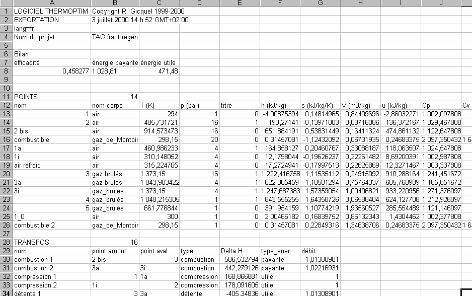
This file comprises the overall balance and the main computation results of the various primitive types which make your project: state of the various points, energies brought into play in the processes, compositions of the project gases...
Point screen
The "point screen" allows one to define a point and to calculate and display values taken by all its state functions. Three modes of presentation exist: by default for open systems, enterable values are pressure and enthalpy; on the other hand for closed systems, one enters the specific volume and internal energy; and finally for water vapor / gas mixtures (a specific section is dedicated to this topic).
For condensable vapors, the software does not calculate the values of specific heats Cp and Cv except in the liquid zone, nor their ratio γ.
Open systems
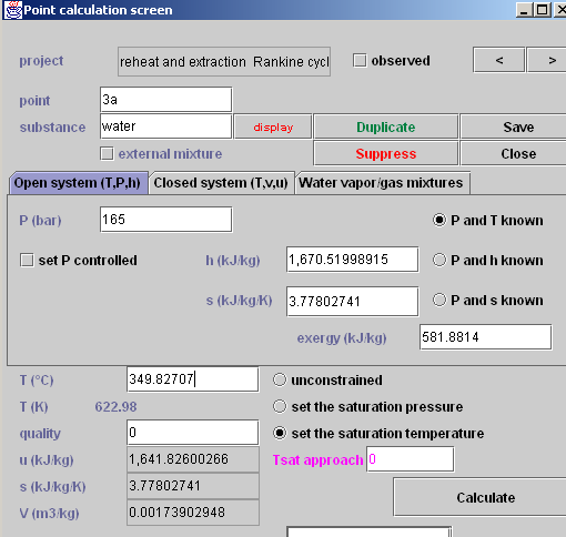
For open systems, the knowledge of the pressure and the temperature allows for the calculation of all the other state functions directly by clicking on the checkbox labeled "p and T known" (the temperature must entered in the unit chosen in the Global properties editor, but it is also displayed in the other unit when the point is calculated). Exergy is calculated on the basis of the reference temperature entered in the Global properties editor. If the pressure and enthalpy are known, select "p and h known". If the pressure and entropy are known, select "p and s known".
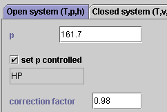
The pressure can be directly entered in the field labeled "p", or set controlled by a pressure setting, if the corresponding checkbox is selected. To select the pressure setting, double-click in the field which appears just below the checkbox, and choose from among the proposed list. It is possible to define a pressure correction factor, by which the pressing setting value is multiplied to calculate the pressure. It is thus possible to automatically take into account pressure drops. In the example shown above, the pressure setting value is 165 bar; as the correction factor is 0.98 (2% pressure drop), the point pressure is set to 161.7 bar.
For condensable vapors are displayed:
- two checkboxes, «set psat» and «set Tsat» which serve to set either the saturation pressure or the saturation temperature
- a field labeled Tsat approach which, used in conjunction with "set Tsat", allows one to set the value of the temperature to (Tsat + Tsat approach). If you set it to 10 K, T will be set to the saturation temperature plus 10 K. If set to 0, T equals the saturation temperature. For instance, if you set Tsat approach to – 5 K, as in this example, T will be set to the saturation temperature (621.33 K) minus 5 K, which gives 616.33 K.
- the quality x of the mix which must be entered in the case when the point is located in the liquid-vapor zone.
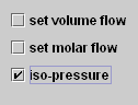
In order to allow one to simultaneously make vary the pressure in a set of points, a specific mechanism has been implemented: the "pressure settings". It is possible to define the pressure settings by associating a name and a value in the frame which can be displayed by double-clicking in the headband of the "Pressure settings" table located in the upper right part of the project frame (e.g. "HP", 165 for High Pressure and 165 bar):
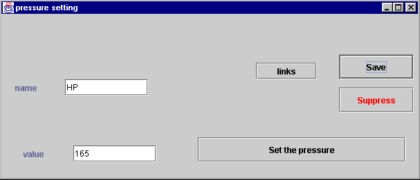
Then, the points which must be at that pressure are connected with this pressure setting. This is done in the point frame by selecting "pressure controlled" and choosing "HP" from among the pressure setting list.
In the point screen, it is possible to define a pressure correction factor, by which the pressing setting value is multiplied to calculate the pressure. It is thus possible to automatically take into account pressure drops. In the example shown above, the pressure setting value is 165 bar; as the correction factor is 0.98 (2% pressure drop), the point pressure is set to 161.7 bar.
When the associated substance is defined, its name appears in the upper left side. To select the substance, you may:
- either double-click in the substance field located in the right side of the screen and expand the substance type folder, then click on the chosen substance (here "Vapors" and then « water »):
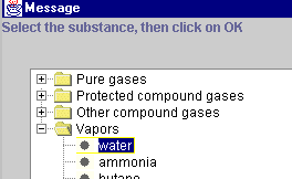
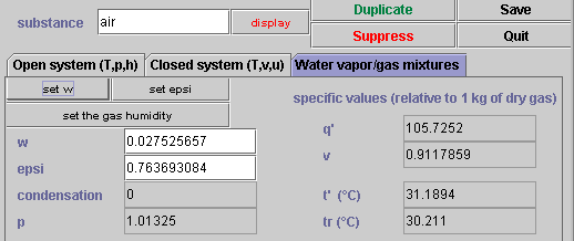
- or enter the requested name in the field and type the "Enter" key. Thermoptim browses through all the existing substances looking for that name. If it exists, it is selected. Otherwise, it considers that you want to create a new gas and opens a gas editor which enables you to select the gas composition from among the existing pure gases (which are shown in a combo-box when you click on a cell of the "component name" column).
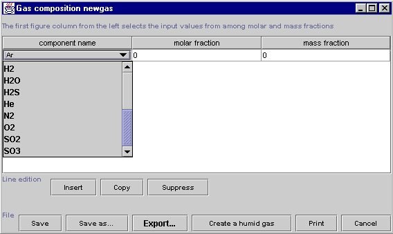
Thermoptim considers that the first column of numbers on the left contains the data to be taken into account, the others being calculated from those (you can move a column by clicking on its headband and dragging it laterally). However, if you choose to enter the mass fractions, it is necessary that the values of the molar fractions are set to 0. Obviously, the sum of the mole or mass fractions must be equal to 1.
Line edition buttons allow you to insert, copy and paste or suppress a line. File buttons allow you to save the gas, rename and save it, export its composition in a text file, create a water vapor / gas mixture of a given absolute humidity, print the frame and cancel the edition. When you are through with entering the constituents, save the compound gas by clicking the corresponding button. If the sum of the molar or mass fractions differs from 1, you are informed by a message and the gas is not saved.
The same gas editor is shown when you click on the "display" button located close to the substance name in the point frame.
If the substance is a vapor, the screen displayed looks as follows:
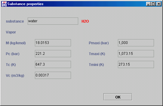
It provides the main characteristics of the substance and the temperature and pressure limits of the model used in Thermoptim.
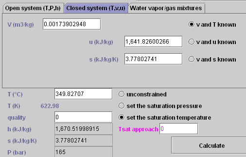
Closed systems
To get access to the closed system screen, click on the middle tab. A slightly different screen is displayed:
For closed systems, the specific volume can be entered, as well as the internal energy, and one can set these two values to determine the other state functions by checking the box "v and u known".
Compound gas editor
The software includes a compound gas editor which we rapidly presented when introducing the definition of a new gas. In this section, we shall give details on the different possibilities of this editor. We have explained previously how a compound gas can be defined or modified. We shall present here the available functions for saving, suppressing, exporting or importing compound gases in the software data base.
You can open several compound gas editors at the same time.
If you display a compound gas, its composition appears in the editor.
You can modify the gas composition, by choosing the constituent names in the list of pure gases which is shown when you click in the first column cells, and entering either the molar or the mass fractions. Once it is defined, the compound gas can be:
- saved, by clicking on "Save". The software checks that the sum of the fractions is equal to 1, and then saves the gas. If the sum differs from 1, nothing is done.
- renamed, by clicking on "Save as…". The test on the sum of the fractions is made, and the gas saved with the new name that you have entered.
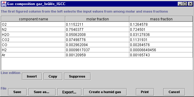
- exported, by clicking on "Export…". The gas composition is then copied in a text file that you name, and that you can open with a spreadsheet or a text editor. For instance, the previous gas can be exported with the following format:
- you can also create, from the gas displayed in the editor, a moist gas of a given absolute humidity. To do that, click on "Create a humid gas". The software asks you to enter the gas name and the absolute humidity requested, and then creates a new compound gas, whose dry gas is the same as that of the gas displayed in the editor, and with the given absolute humidity. This gas is added to the list of compound gases of the data base. You get access to it by the previous screens.
- lastly, if you cancel, the compound gas editor is closed.
Process screens
All process screens are similar:
- in the upper left zone is the process name
- in the upper right zone are located a number of fields and checkboxes which are used to set the process parameters: open or closed system, set flow process, observed process (these two notions are used for controlling the automatic recalculation engine. Their precise meaning is explained below in the section devoted to this topic).
- in the left side appear the inlet and outlet points, their main state variables being displayed. To connect the inlet point, double-click in the inlet point field, and choose from among the list of points which is proposed in a combo box. Do similarly to connect the outlet point.
- the type of energy (useful, purchased or other) corresponding to the process can be modified by double-clicking in the energy type field).
- the mass flow-rate value can be entered in the upper zone. By default it is set to 1. The unit is not indicated purposely, so that the user may consider mg/s, g/s or kg/s depending on the problem studied while keeping a good display accuracy. It is obvious that the calculation results concerning enthalpies and energies depend on the flow rate unit and may be expressed in mJ (mW), J (W) or kJ (kW). If you check the "set flow" box, the value you enter will be set. Otherwise, it will be automatically changed by THERMOPTIM if there is only one process connected at the inlet (refer to the recalculation engine section for more details).
- the parameters which are process-type specific are shown in the right part of the screen.
- the "links" button allows one to display the link browser frame.
- finally a text field allows one to enter a description of the process.
Compression and expansion


The screen displayed is about the same for both processes.
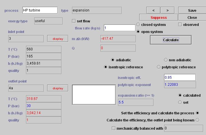
For compression and expansion, possible choices are the following:
- calculations can be made either for an open system, in which case they focus on the pressure and the enthalpy, or for a closed system, in which case it is for the specific volume and internal energy.
- the compression ratio ρ can be set, in which case the pressure (or the specific volume) of the outlet point is determined from that of the inlet point and the value of ρ chosen, or calculated, in which case the value of ρ is evaluated from pressures or volumes of inlet and outlet points, considered as data. In all cases, be it for a compression or an expansion, ρ is superior or equal to 1.
- the process can be adiabatic or polytropic. Accordingly, it is characterized by an isentropic or polytropic efficiency, between 0 and 1.
When it is adiabatic (checkbox "non adiabatic compression" or "non adiabatic expansion" unchecked), it is characterized by an isentropic or polytropic efficiency, in the range 0 to 1. In this case the polytropic exponent k of law is calculated by Thermoptim.
When it is non adiabatic, the process is polytropic and characterized by its polytropic exponent n, and its polytropic efficiency (for a compression, it is the ratio between the reversible work and the real work, for an expansion the inverse). In this case the heat Q exchanged with the surroundings is calculated by Thermoptim and displayed in the field located below the compression or expansion work Delta H or Delta U.
One should make sure not to confuse the polytropic efficiency ηp with the polytropic exponent k. For a poytropic expansion in open system, these two values are related by equation:
Two complementary calculation modes are accessible on this screen:
- "Set the efficiency and calculate the process" initiates the calculation of the outlet point state, from that of the inlet point and of the compression or the expansion characteristics.
- "Calculate the efficiency, the outlet point being known" allows one to identify the value of the compression or expansion efficiency corresponding to the outlet state.
Heat exchanges


The screen is similar to the previous one, just a little simpler, as the options are less numerous:
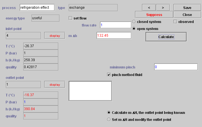
An « exchange » process serves to calculate the heating or the cooling of a fluid between two states represented by inlet and outlet points. Two « exchange » processes can be matched to form a heat exchanger.
In the right, appears a field that allows one to define the minimum pinch for this fluid. This parameter can be used for the design of heat exchangers. A checkbox (selected by default) allows to select this process as one of the fluids to take into account when running the pinch optimization method (refer to the Optimization method section for more details.
The two checkboxes in the lower right frame are settings for the calculation method:
- «Calculate Delta H, the outlet point being known » evaluates the enthalpy involved in the process
- «Set Delta H and modify the outlet point» calculates the outlet point temperature so that the enthalpy involved in the process is equal to the value entered in the Delta H field.
volumetric and molar flow rates
In version 1.5, it is possible to display or hide the volumetric and molar flow rates. To display them, select the option “Display volumetric and molar flow rates” from the global preferences screen (Help menu).
You can then enter the set flow rates in volumetric and molar values in all of the process-points and exchange processes, which can be useful in a number of instances.
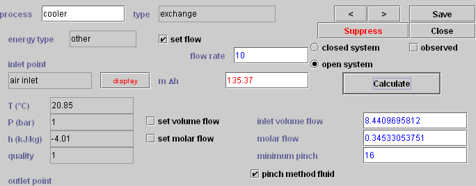
To allow users to input volumetric and molar flow rates, the “exchange” process and process-point screens have been changed
Two fields and two options have been added. You can enter either the volumetric flow rate or the molar flow rate (by default the mass flow rate is used). In all cases, the two non-specified flow rates are calculated based on the third.
In order to avoid conflict with the automatic flow rate propagation system, you can only choose the set volumetric flow rate or set molar flow rate options in processes with set flow rates. If you select one of these two options and the flow rate of the process is not yet set, a message will appear asking you to check that the set flow rate option is consistent with your model, then the flow rate is set and you cannot change this choice, unless you deselect the set volumetric flow rate or set molar flow rate options.
“Exchange” processes can also be made isobaric. To do so, first select the “Isobaric exchange processes” option on the global preferences screen (by default it is not selected). Once this option is selected, the “exchange” processes screen displays an isobaric option, checked by default when a process is created, and saved in accordance with the user’s choice. When this option is visible and checked, the pressure of the upstream point is automatically propagated to the downstream point. Otherwise, nothing is done.
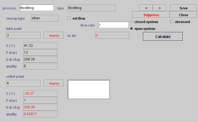
Throttling

The Throttling screen is among the simplest, as the only calculation which can be made consists of determining the temperature, the quality and the entropy of the outlet point knowing that the throttling is isenthalpic.
Combustion

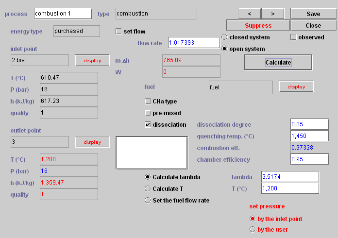
The combustion screen is the most complex, as the options are numerous.
Fuel declaration
When air is in excess, the complete non stoichiometric combustion reaction of the fuel CHa with air can be written as function of the air factor λ:
THERMOPTIM uses a generalized equation of this kind, where the oxidizer can be any compound gas containing oxygen, and the fuel can be either given under the form CHa, or declared as a substance included in the database.

The fuel definition is made in the upper right of the screen:
If it is a substance included in the database, the fuel is a pure or compound gas containing any of the following reactants: H2, CO, H2S, CnHmSpOq, n, m, p and q being decimal less than 100. Inert gases taken in account are: Ar, CO2, H2O, N2, SO2. To connect the fuel, double-click in the fuel field, and choose from among the list of processes which is proposed in a JComboBox.
The fuel and oxidizer both can be composed of reactants, oxygen and inert gases, even if usually the fuel does not have any oxygen, nor the oxidizer any fuel. It is thus possible to study complex combustions, such as vaporized mixes made before they are introduced to the combustion chamber.
The reaction products are the following: CO2, H2O, SO2, as well as CO and H2 if there is dissociation, and fuel if the reaction is not complete.
The software analyzes chemical component formulae of the fuel and the oxidizer, and deduces the reaction that takes place. Calculations can then be executed. For the time being, chemical formulae are obtained by analyzing substance names.
When the fuel is a substance included in THERMOPTIM, the name that appears on the screen (here «fuel») has to be that of a process (for example a process-point); this allows one to specify its flow rate. This process is itself connected to a point specifying the name and the state of the substance (pressure, temperature).
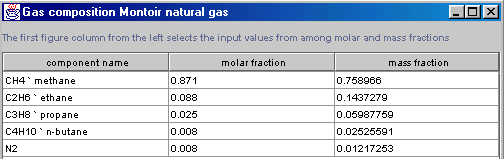
The example below is taken from the Getting Started example n° 2 « gas turbine ». It relates to the natural gas available at the LNG terminal of Gaz de France at Montoir de Bretagne (France) and illustrates how to declare a fuel whose composition is the following:
Each constituent, except for the nitrogen, is a fuel, whose chemical formula appears in first part of the name that sometimes is followed by a comment, separated from the formula by the character « ` ». By analyzing the chemical formula of each constituent and its molar fraction, THERMOPTIM completely characterizes the fuel.
This substance is associated to a point, allowing specification of its temperature, which is taken into account for the calculation of the outlet gas temperature. The flow rate is associated with a process-point, whose name serves as parameter for the combustion.
When the fuel is given in the form CHa, it is necessary to enter the values of a, and of its enthalpy of formation hf0 (relative to the formulation CHa). It is then impossible to specify the flow rate.
Open systems and closed systems
It is necessary to specify if the combustion takes place in an open or closed system. For open systems, the pressure must be set to a certain value. It can be done either «by the user», which means that this value will be that of the outlet, or «by the inlet point», which corresponds to a constant pressure combustion equal to that of the inlet oxidizer.
For closed systems, one can choose between three possibilities: set the volume, set the pressure, or constant temperature combustion. For the two first cases, two different modes of setting the volume or the pressure exist: «by the user» or «by the inlet point». In the third case, the combustion temperature is constant and equal to that of the inlet oxidizer.
In the two last cases (set pressure and constant temperature), the volume varies with combustion, so that a part of the energy liberated by the combustion transforms directly into mechanical energy due to the expansion of the volume.
The first law of thermodynamics indicates indeed that internal energy variation (du) is the algebraic sum of the heat (dQ ηcbst ηth) and the work (dW = - pdv) received by the system.
THERMOPTIM calculates the W value and displays it just below the value of the energy liberated in the combustion. This value is subsequently taken into account as a useful energy when the cycle balance is calculated. One can refer, for more understanding of this subject, to the example n° 4 on diesel and spark ignition engines presented in the User’s Guide.
Setting the combustion
The dissociation of CO2 in CO can be taken in account by clicking on the appropriate button, and by entering the corresponding dissociation degree. In the case of air, the combustion reaction becomes :
The dissociation of CO2 is given by equation:
This equilibrium does not depend on the pressure: it is a function of temperature only. With the hypothesis that combustion kinetics are fast enough for equilibrium to be reached, the mass action law gives:
THERMOPTIM calculates the dissociation using a similar but generalized approach.
In case of dissociation, a field is displayed in which must be entered the dissociation degree k1 and the quenching temperature Tq which are used in the calculation of the constant Kp.
- to take into account possible thermal losses of the combustion chamber, which may be non adiabatic, one introduces a thermal efficiency ηth whose default value is set to 1 (left to the center of the screen). This efficiency differs from the combustion efficiency ηcbst, calculated by the software as function of the dissociation degree and the quenching temperature.
In the lower left part of the screen appear two enterable fields, corresponding on the one hand to the air factor λ, and on the other hand to the outlet gas temperature Tgo. It is possible to set either of these values, and calculate the other. The air factor can be greater or smaller than 1. If it is smaller than 1, the software will assume that it represents an air default combustion forming carbon monoxide CO. If the air factor is too small for all available carbon to be oxidized in CO, a message warns the user.
Calculation options
- the checkbox «Calculate T» determines the outlet gas temperature Tgo, from the value set for λ. The mass flow rate of the combustion process is set equal to the sum of fuel and oxidizer flow rates, which means that the combustion process behaves, at the hydraulic level, as a flow rate mixer.
- the checkbox «Calculate lambda» determines λ (≥1), from the value of Tgo set. Flow rate calculation rules are analogous to those of the preceding button.
When the combustion is calculated, values of the combustion efficiency and of the fuel LHV are also determined. The chamber efficiency is used to take into account the non adiabaticity of the combustion chamber. In order to make sure that the energy conservation law applies to the combustion, THERMOPTIM multiplies the heat liberated by the combustion by the chamber efficiency for calculating the outlet gas temperature Tgo (which therefore differs from the adiabatic flame temperature)
Particular case of pre-mixed reactants
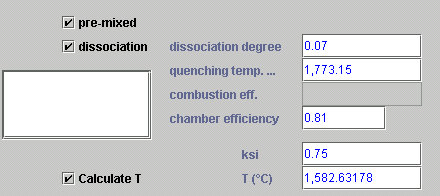
As indicated above, it is possible to combust a reactant mix that is prepared before it is introduced to the combustion chamber (for example a fuel-air mixture prepared in a carburetor, which can be easily modeled in THERMOPTIM by a Mixer node). In this case, there is no longer a need to specify a fuel that is present in the oxidizer. In order that the software knows that this is the case, it is necessary to choose the option « type CHa », and set the values of a and hf0 to zero. Note: this is what had been implemented in the 4D version, but it could be preferable to add a special checkbox for pre-mixed reactants).
As it is clear in this case that the notion of air factor λ loses its meaning, this parameter is used to represent the burnt fraction of the reactants ξ. If ξ < 1, one assumes that only a fraction ξ of the mix has reacted, and that (1- ξ) has not reacted. Combustion gases are then considered as a dual gas mixture: one the reaction products, including inert gases, and two the fraction of the initial mix that has not reacted. This allows one to start from a given mix, and to separate its combustion in several phases, for example constant volume, then constant pressure, then constant temperature. One can refer, for more understanding of this subject, to the example on spark ignition engines.
Node screens
A node screen is roughly divided in three parts:
- the upper left one displays information relative to the node main process (the outlet one for a mixer, and the inlet one for a divider or a separator). To connect it, double-click in the main process field, and choose from among the list of processes which is proposed in a combo box.
- the lower left one shows the branches of the node
- the right part shows the actions which can be taken for building the node
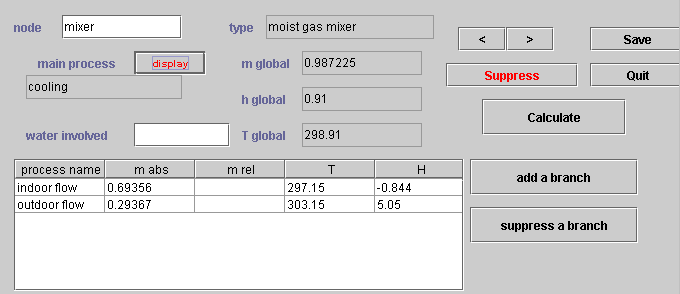
Mixer

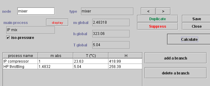
In a mixer, you can either add or remove branches. When the node is built, the "Calculate" button allows one to make the mass and enthalpy balance and calculate the outlet temperature. The inlet point of the process connected at the outlet of the mixer is recalculated.
Divider

The divider screen shows an additional button labeled "flow setting". This feature allows one to define the flow factor which will be taken into account for calculating the flow distribution between the branches.
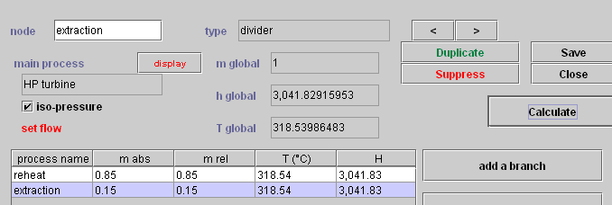
The basic idea is the following: as a divider must conserve the mass flow rate, it is not possible to set the value in the different branches if that of the main branch varies. Therefore the user defines in each branch a "flow factor" which represents the share of the given branch in the global flow rate.
THERMOPTIM then adds the different flow factors and distributes the main flow-rate between the branches proportionally to their "flow-rate factors". In the example presented above, 25 % of the flow rate goes to the extraction process, and 75 % to the resuperheating one.
There is however an exception: it is possible to set the flow rate in a process at the outlet of a divider, provided that this node has two branches, that with the set flow rate, and another one. In this case the flow rate of the second process is set equal to the flow rate of the main vein, minus that of the branch with the set flow rate, and the flow-rate factors are recalculated accordingly. In this case (as in the previous example) the message "set flow" is displayed in red below the name of the main vein.
Separator (dryer)

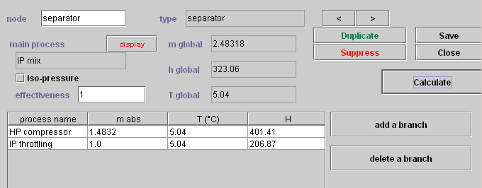
As its name indicates, its role is to separate a fluid in a liquid-vapor equilibrium, characterized by its temperature, pressure and quality. This is done by dividing its flow rate into two parts, liquid and vapor. It is therefore a type of divider.
To create a separator, select the process that represents the diphasic fluid. The outlet point of this process has to be diphasic, which means that its quality has to be strictly between 0 and 1. If this is not the case, the separator cannot be calculated and a message warns the user.
Select then the two outlet processes, which must have inlet points whose substance is the same as that of the main process outlet point. Furthermore one of these two processes must have its inlet point quality set to 0 so that THERMOPTIM may identify it as being the liquid vein.
You may set a separator effectiveness which must be in the range 0 to 1. It is defined as the ratio of the real liquid flow rate to the maximum theoretical one, and thus represents a drying effectiveness. If it is lower than one, the value of the quality of the vapor exiting the separator is less than 1.
Heat exchanger screens
The heat exchanger calculation screen has in its central zone two parts, the one on the left for the hot fluid, and the one on the right for the cold fluid. Besides values of temperatures, flow rates, specific heats and enthalpies involved, there appear constraints on temperatures and flow rates that serve to guide heat exchanger calculations by allowing one to distinguish from among the problem variables those that are set and those that have to be calculated.
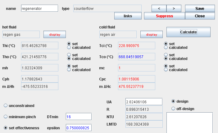
The following are possible types of heat exchangers: counter-flow, parallel-flow, crossed flows, mixed or unmixed Cpmin or Cpmax, and (p-n).
In the lower left corner, appear:
- three checkboxes allowing one to specify the absence or presence of implicit constraints on temperatures (see below).
- A field for entering and/or displaying the value of the effectiveness
In the lower right corner, appear:
- two checkboxes for setting the heat exchanger calculation mode: either "design" or "off-design".
To connect the hot or the cold fluid, double-click in the corresponding field and choose from among the list of exchange processes which are proposed.
Design of simple heat exchangers
A heat exchanger connects two « exchange » processes. One of them is a hot fluid which corresponds to a substance that gets colder, while the other is a cold fluid that gets hotter.
Once the coupling of the processes is made, the design problem is the following: it is necessary on one hand to conserve enthalpy in the heat exchanger, and on the other hand to respect some temperatures constraints.
Given that there are four temperatures (two for each fluid) and two flow rates, the problem has five degrees of freedom once the enthalpy is conserved. One can furthermore show that at least one of the two flow rates has to be set, otherwise the problem is indeterminable.
For temperatures, one can either set explicit constraints (for example temperatures of the inlet fluids), or implicit constraints (the value of the heat exchanger effectiveness, or the pinch minimal value).
To set a value to the effectiveness, enter the value in the ε field, and click on the button «set effectiveness». To set a «minimal pinch», click on the corresponding button. The minimal pinch value is initialized, when the heat exchanger is created, or when one double-clicks in this field, with a value equal to the half sum of the minimum pinches defined in both hot and cold processes. The user can thus either keep this value or enter another one. When the heat exchanger is calculated, the pinch is set equal to the value which appears in this field.
For the problem to have a solution, it is necessary to set a total of five constraints, among which there is a flow rate. If one of them is implicit (effectiveness or minimal pinch), four have to be explicit (3 temperatures and 1 flow rate, or 2 temperatures and 2 flow rates), or otherwise all five have to be explicit (a single flow rate or a single temperature is free).
These conditions are necessary, but non sufficient. This is why THERMOPTIM analyzes all the constraints proposed. If there is a solution, it will be found. Otherwise, a message tells the user that the calculation is impossible.
It should be noted that it is recommended to avoid that the exchange processes that are coupled by a heat exchanger are parameterized according to the "Set Delta H and modify the outlet point" mode, because this configuration can lead to a conflict between the solutions calculated by the exchanger and by the process.
One can note that the design of heat exchangers is always made with the implicit hypothesis that thermophysical properties of the fluids remain constant in the heat exchanger, but this hypothesis is not made during the calculation of the processes. Therefore, when one recalculates a temperature on the basis on heat exchanger equations, slight differences may exist between the values displayed on the heat exchanger screen and that of the corresponding processes, or between the values of the enthalpies involved in both hot and cold fluids. If a high accuracy is required, one may have to make first a heat exchanger design calculation, and then iterate. Convergence is obtained fast.
When a heat exchanger is designed, one of the flow rates being calculated, that of the exchange process is recalculated, as well as those of the processes located upstream as long as they are straightly connected. The propagation stops when a node or a combustion process is encountered.
Generic liquid
Let us recall that a particular substance called «generic liquid» exists in the database. It is a liquid at atmospheric pressure, whose specific heat is equal to 1 kJ/ kg/ K. It can be used to simulate any liquid not included in THERMOPTIM that one wants to use in a heat exchanger.
Indeed, in the energy equations used for calculating heat exchangers, the flow rate m and the specific heat Cp always appear as their product mCp, sometimes called the calorific flow rate. Therefore, if Cp is set equal to 1, the value which is displayed in the flow rate field of the heat exchanger form is that of the product mCp.
Instead of entering in the database a large number of different liquids, it is thus possible to make use of a single one: the generic liquid.
Suppose that you want to study a liquid whose specific heat is Cpliq.
If the liquid flow rate is set to mliq, enter in the exchange process flow rate field the value (mliq.Cpliq). Set the other constraints and calculate the heat exchanger.
If the liquid flow rate is to be calculated, set the other constraints and calculate the heat exchanger. The value of the liquid flow rate will be equal to the value returned by THERMOPTIM in the flow rate field, divided by Cpliq.
Solving non nominal operation for heat exchangers
THERMOPTIM allows one to calculate non nominal operation of the heat exchanger by the NTU method if at least two temperatures are known.
For automatic recalculation, causality rules imply that the inlet temperatures and the mass flow-rates of the hot and cold fluid be known, and THERMOPTIM sets them from their processes (see the recalculation engine section for more details). Step by step calculation offers more flexibility in this regard.
All non nominal operation procedures apply to the study of a pre-designed heat exchanger. One notes that, to use the NTU method, one implicitly makes the hypothesis that the thermophysical properties of the fluids remain constant in the heat exchanger.
The procedure updates inlet bounds of the module, starting from the processes, then calculates the outlet temperatures, and balances the heat exchanger at the enthalpy level. Points and processes associated to the module are updated as a function of the results.
For the time being, no correction is made on exchange coefficients when flow rates are non nominal.
Water vapor / gas mixtures
From now on, we call "humid gas" or "moist gas" a substance that is composed of one or several pure gases and water vapor which may condense. In these conditions, the composition of the mix can evolve even in simple cooling processes. Therefore, as explained below, the processes generally defined in THERMOPTIM do not always allow one to determine the thermodynamic properties of humid gases.
In practice, the most frequent case is obviously that of moist air at atmospheric pressure, and THERMOPTIM allows one to solve many air conditioning problems. But more generally, it allows for study of any water vapor / gas mixture such as combustion flue gases.
A hypothesis however must always be made: the gaseous water is supposed to behave as an ideal gas, which means that its partial pressure remains inferior to a pressure level of a few bars; this is almost always the case.
To calculate thermodynamic properties (essentially enthalpy) of a humid gas, it is practical to apply the Dalton’s Law knowing that it concerns a two constituent mix: the dry gas (possibly a mix of gas itself), and the gaseous water.
Furthermore, in THERMOPTIM the zero level, or reference state for calculations of gas enthalpies is standard, chosen at 298 K. However, air conditioning engineers have chosen that the saturated-liquid state is at 0 °C for steam, and 0 °C for dry air. This leads to a difference between the humid gas enthalpy as calculated in THERMOPTIM and that used in psychrometric charts. This difference varies according to the specific humidity.
Another point has should be noted: in THERMOPTIM, point thermodynamic properties are expressed in mass units for intensive values.
However, in most of water vapor / gas processes, the total mass of the gaseous phase does not remain constant, due to the variation of the water content of the mix. The single invariant in these conditions is the dry gas mass, to which it is customary to relate the point properties. The qualifying of "specific" means that expressed values pertain to 1 kg of dry gas, when considering humid gases.
Finally, the enthalpies that will be considered later can be related to three different references:
- mass enthalpy of the dry gas hgs (hgs = 0 at T = 298 K)
- mass enthalpy of the humid gas hgh (hgh = 0 at T = 298 K)
- specific enthalpy of the humid gas q’ (q’= 0 at T= 0 °C, liquid water)
With usual notations, w being the specific humidity of the gas, these three enthalpies are connected by the following equations:
q’(t,w) = hgs(t) - hgs(0 °C) + w (hH2O(t) - hH2O(0 °C)) + w L0water
q’(t,w) = (hgh(t) - hgh(0 °C)) (1 + w) + w L0water
hH2O(t) being the enthalpy of the gaseous H2O as calculated by THERMOPTIM, and L0 water the heat of vaporization of water at 0 °C.
One can therefore represent a humid gas in THERMOPTIM in two equivalent ways: either directly as a substance composed of at least two constituents: H2O and another gas, pure or compound, or as a dry gas whose specific humidity is known. The first manner presents the advantage that the composition of the humid gas is accessible at any time. The drawback is that, for a given dry gas, one has to create a new humid substance for each value of the relative humidity. Furthermore the second representation is far more concise, as the only substance required is that of the invariant gas.
Let us finally note that water can be present three states, solid, liquid, or gas, according to the temperature and the humidity of the gas considered. However, for practical reasons, the lowest temperature of water vapor / gas mixtures has been set to - 123 °C or 150 K in THERMOPTIM.
Point screen
The water vapor / gas mixture screen gives access to procedures for analyzing humid gases. When the gas is represented by a humid substance, it could have been mixed in a mixer, generated from a dry gas and a specific humidity, or again directly defined by the user, in which case the water has to be entered as a gas (H2O).
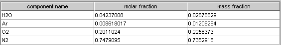
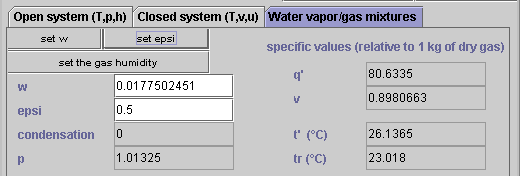
For example, let the humid air have the following composition:
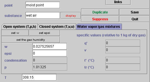
Build a point using this substance, at the pressure of 1 atmosphere and a temperature of 35 °C, calculate it and click on the tab "water vapor / gas mixtures". The following screen appears:
The specific humidity w of the point considered appears. As the gas is a moist gas, Thermoptim automatically calculates it and displays it on the screen.
Specific values (i.e. related to 1 dry gas kg) of enthalpy and volume are also shown, as well as the humid characteristics: possible condensation, humid temperature t' , dew point temperature tr..
When this screen is displayed, values of the relative humidity epsi, condensation, dew point temperature, specific enthalpy and volume are put to zero.
Humid characteristic calculations
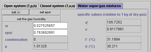
To calculate all the humid characteristics of the point, click on the button "set w". The following results are displayed:
Setting the relative humidity
It is possible to set the relative humidity to a particular value, by entering the value in the corresponding field, and then by clicking on the button "set epsi". In this case, the water content of the humid gas is modified to obtain the desired value and the humid characteristics are updated.
Suppose now that one sets a relative humidity equal to 0.5:
By clicking on "set the gas humidity" you can change the gas composition and obtain the following result:
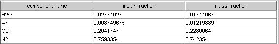
If the quantity of water present in the mix exceeds the saturation content, the relative humidity has the value 1, the specific humidity becomes equal to the saturation humidity, and the quantity of water in excess appears in the field titled "condensation".
In the Thermoptim 4th Dimension version existed two ways of representing the gas, either as a moist gas or as a dry gas. In the Java version, all humid calculations are made on the basis of the dry gas properties and it is not any more necessary to distinguish between both cases.
For instance, if you select the gas "air" instead of "wet air" and enter the same value for w as in the first example, you obtain the following result:
The values obtained with the dry gas are the same as with the moist gas.
Water vapor / gas mixtures process screens
"Water vapor / gas mixtures" processes correspond to six different processes that distinguish by their category. The water vapor / gas mixtures process screens are as follows ; they vary slightly according to the category chosen:
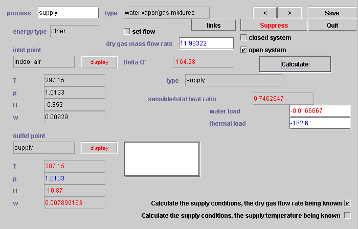
This is for when a "supply" process is involved. It calculates supply conditions for maintaining a desired ambiance and considers water and thermal loads.
Before explaining how to use this screen, let us specify some general issues pertaining to the water vapor / gas mixtures processes.
First of all, THERMOPTIM calculates processes between humid points on the basis of their dry gas properties. As stated before, the reason is simple: this mode of representation avoids introducing a new humid substance for each value of the relative humidity.
Secondly, values are expressed preferably in specific units. Flow rates that appear on the processes are dry gas flow rates and enthalpy variations Delta Q' relate to specific enthalpy.
Efficiencies are often used to qualify the real processes in comparison to the theoretical or ideal processes. In practice, they generally correspond to evolutions whose final state is saturated (complete humidification, cooling until saturation).
The right and upper sides of the screen display general characteristics of the process, while the left side displays inlet and outlet points, their specific humidity w being displayed. In the right are given values of the "sensible/total heat ratio", and of the total enthalpy involved in the process (on the basis of the specific enthalpies), as well as the settings of the different categories of water vapor / gas mixtures processes, and in the lower part the calculation options.
Supply process
The supply process connects the point describing the known internal ambiance (inlet point) to the point corresponding to the supply conditions sought out (outlet point).
The enterable fields allow one to enter the thermal load and water load to remove, in kW and kg/s respectively, which defines the supply line. One makes the hypothesis that the water load has to be removed at the inlet point temperature.
The two possible options are in this case:
- to determine the temperature and the specific humidity of the supply point when the dry gas flow rate is known.
- to set the supply temperature, so that THERMOPTIM determines the specific humidity of the supply point, as well as the dry gas flow rate required.
Cooling process
The cooling process allows one to study humid gas cooling in a cooling coil, with or without condensation.
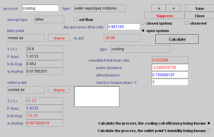
Cooling conditions are specified in the right of the screen: surface temperature and effectiveness of the cooling coil, if they are both known. If the effectiveness is not known, the outlet point humidity allows for the calculation of the process.
The two possible options are in this case:
- to set the effectiveness, in which case THERMOPTIM calculates the specific humidity of the outlet point. In case of anticipated condensation (the case when the line connecting the inlet point to the point of the saturation curve at the surface temperature cuts the saturation curve twice), the outlet point is located on the saturation curve and its enthalpy is calculated from the effectiveness of the coil.
- to set the specific humidity of the outlet point, in which case THERMOPTIM calculates the coil effectiveness. In the case of anticipated condensation (see above), the outlet point is located on the saturation curve, at the desired specific humidity.
Vapor or water / adiabatic humidification process
This process allows one to study either water or vapor humidification or adiabatic humidification.
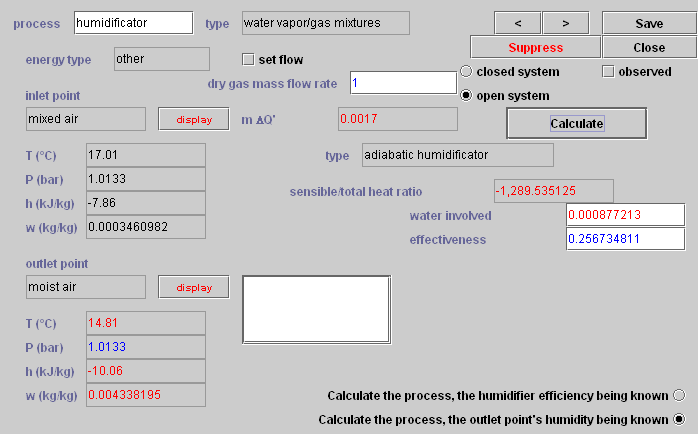
Humidification conditions are specified in the enterable fields: water or vapor temperature and pressure, and humidifier effectiveness, if it is known. If the effectiveness is not known, the value of the specific humidity of the outlet point allows for the calculation of the process.
The two possible options are in this case:
- if the effectiveness is set, THERMOPTIM calculates the humidity of the outlet point. In case of anticipated condensation (see above), the outlet point is located on the saturation curve and its enthalpy is calculated from the humidifier effectiveness.
- if you set the specific humidity of the outlet point, THERMOPTIM calculates the effectiveness of the humidifier. In case of anticipated condensation (see above), the outlet point is located on the saturation curve at the desired specific humidity..
Desiccation process
The desiccation process allows one to study dehumidification by desiccation or the regeneration of a desiccant material. Different types of desiccant materials are presented. Their name and their sorption heat value are displayed in the right part, the latter being enterable by the user.
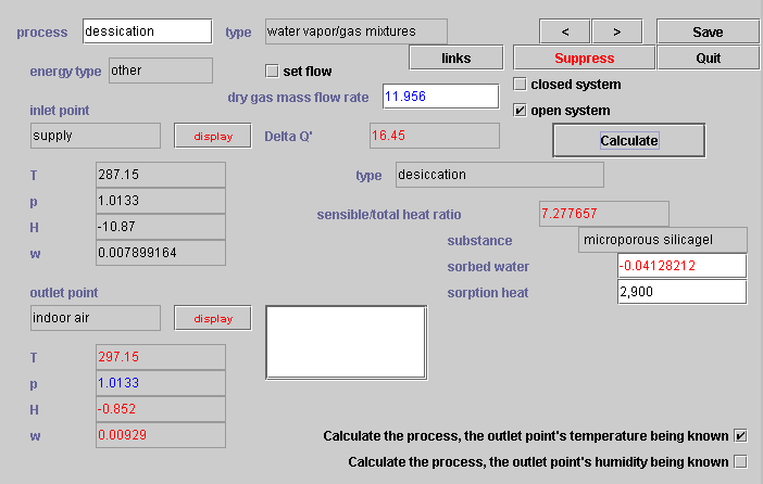
The two possible options are in this case:
- if the outlet point temperature is known, THERMOPTIM calculates its humidity.
- if you set the specific humidity of the outlet point, THERMOPTIM calculates the outlet point temperature.
One should note that the same process calculates the desiccation as well as the regeneration of the desiccant, according to relative values of the inlet and outlet points. For regeneration, the software unfortunately does not verify if the temperature is high enough.
Heating process
The heating process allows for different calculations of a humid gas. It connects two points whose water contents may or not be the same.
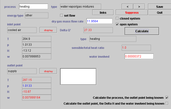
The two possible options are in this case:
- if the outlet point is set, THERMOPTIM calculates the Delta Q' and water involved.
- if you set the specific enthalpy variation Delta Q' and the water involved, THERMOPTIM calculates the outlet point temperature.
Moist mixers
The moist mixer allows one to determine humid properties of a mixture of streams that may be composed of various dry or humid gases with different water contents.
The moist gas mixer differs from regular mixer in the following way:
- first, it accepts as inlet branches both moist processes and other processes. As the moist process flow rate relates to the dry gas whereas the other process flow rate does not, the moist gas mixer takes this difference into account when it calculates the mix.
- second, its main vein must be a moist gas process. If it is not the case, a message warns the user and the calculations are made as for a regular mixer.
The calculations are similar to those of a regular mixer. In addition, the moist gas mixer checks whether the mix is oversaturated or not. In case of oversaturation, a message warns the user and THERMOPTIM researches the mix point on the saturation curve, by conserving the enthalpy. The excess water is then displayed above the branch table.
The global values which are displayed do not refer to specific values.
Diagnosis tools
Remember that in version 1.5 and later, the interface between the diagram editor and the simulator has tools for identifying and deleting modeling errors.
By modeling errors, we basically mean inconsistencies between the two working environments:
- elements of the simulator absent from the diagram editor
- elements of the diagram editor absent from the simulator
- unconnected points present in the simulator
- unused substances
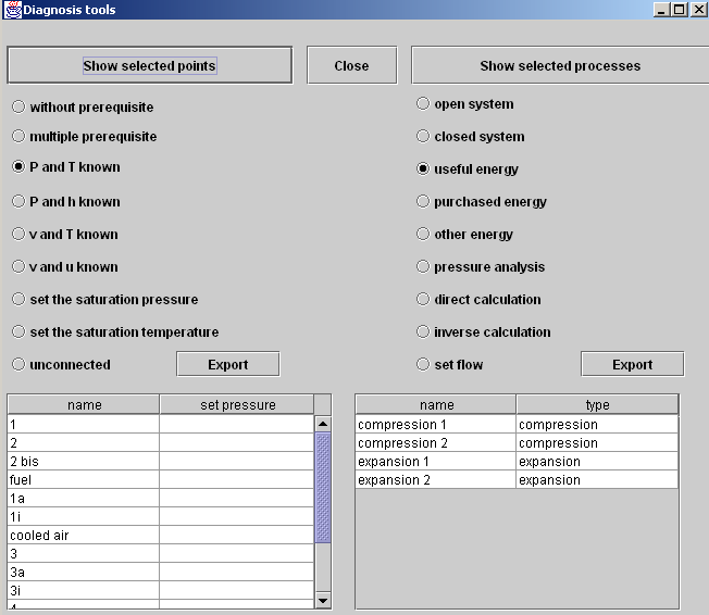
The “Diagnostic Tools” screen also facilitates model checking (in the Standard version and higher). It is accessed from the Special menu of the main project window.
It is comprised of two tables. On the right part of the screen you may select a process search criterion from a list (open or closed system, useful, purchased or other energy type, direct or inverse calculation, set flow rate). Once a criterion is selected, clicking the button "Show selected processes" loads the table located in the lower right part of the screen.
The list on the left side is similar. It allows you to display the points corresponding to the selected criterion (without any prerequisite other than the associated substance or a pressure setting, open system, p and T or p and h being known, closed system, v and T or v and u being known, set saturation pressure or temperature). If the point pressure is set, the pressure setting name appears in the right column of the table.
Both tables are double-clickable : if you double-click in one of them, the corresponding point or process is displayed.
If you click on button "Export" the list of the points or processes is written in file "output.txt".
For points, the search options are as follows:
- no prerequisites other than the substance that is linked to them or a set pressure: theoretically, these points are never modified, unless the composition of the linked substance changes or if the set pressure is changed.
- multiple prerequisites: if a point has more than one prerequisite, it means that it can be modified by more than one component. This is generally because, during modeling, it was incorrectly connected either to the outlet of two different transformers, or to the outlet of one transformer and the inlet of the main transformer of a mixer.
- calculated in open system with either p and T or p and h known.
- calculated in closed system with either v and T or v and u known;
- with a set saturation pressure or a set saturation temperature;
- not connected to a process: these points are not used and can generally be deleted.
For processes, the search options are as follows:
- open or closed system;
- type of energy: useful, purchased or other;
- pressure analysis: in Thermoptim, the pressures are initialized by default at 1 bar, then the user must set the values, since the software does it in only a very few instances. If the user forgets to do so or makes an error, convergence problems may appear. This search option covers on the one hand all of the processes other than compression, expansion and throttling in which the outlet pressure is either greater than the input pressure (physical impossibility except for certain external processes), or less than 80% of the inlet pressure (excessive pressure drop), and on the other hand all of the nodes through which the pressure increases (physical impossibility except for certain external nodes).
- direct or reverse calculation;
- set flow rate: this option facilitates checking of flow rate propagation consistency in complex projects.
You can double-click on the two tables. If you double click on one of the lines, the corresponding components are displayed. By clicking on “Export”, you print the list of points or processes to the file “output.txt”.
In the screen shot above, there is 1 point with multiple prerequisites, and the right part of the screen shows the result of a pressure analysis.
Point with multiple prerequisites
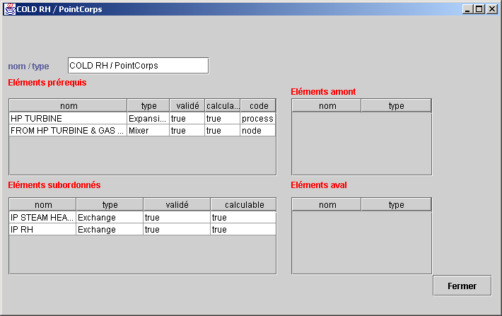
Double click on the line of the point “COLD RH” to display its screen and access the links window (see the paragraph “Links Browser” in the next section).
By looking at the prerequisite elements, we see that that “COLD RH” is defined both as an outlet point of the “HP TURBINE” turbine and as an inlet point of the main process of the mixer “FROM HP TURBINE & GAS…”, which is a modeling error that would have been difficult to detect without the diagnostic tool.
Pressure analysis:
The pressure analysis has identified six components that may have incorrect parameter settings. Double click on the table on the right to display their screens. For the first three, the outlet pressure was rounded up, and the error is negligible.
The next two components are external processes corresponding to a non-adiabatic compressor and a non-adiabatic turbine, so it is perfectly normal for the first component’s downstream pressure to be greater than its upstream pressure, and for the second component’s downstream pressure to be less than 80% of its upstream pressure.
As for mixer “MIX2”, the pressure upstream of its main process is greater than the downstream pressure of its branches, which is clearly an error in parameter setting.
Thus, the diagnostic tool identified three negligible errors, two normal pressure changes in external processes, and one parameter setting error at the outlet of a mixer. Since the project involves sixty or so points and processes as well as fifteen or so nodes, identifying these errors would have been difficult without this tool.
Automatic recalculation Engine
Introduction
Thermoptim allows for the calculation of complex thermodynamical systems. As we saw it above, an analysis of the main different energy technologies shows that it is possible to model most of them using a limited list of basic functional elements which are called primitive types and will sometimes be referred to as "types" in this document. Thermoptim is precisely built on such a primitive type set:
- fluid properties are represented by two kinds of substances, ideal gases and vapors
- the full state (pressure, temperature, enthalpy, entropy, volume,…) of a substance can be calculated within a point, when two state variables are known.
- fluids undergo changes in the different elements of thermodynamical machines, which are called processes (compressions, expansions, exchanges, combustions, throttles, moist gas processes…). Processes connect together at least an inlet and an outlet points.
- fluids flow in the machine elements through a more or less complex network of ducts. Processes represent simple ducts arrangements. For more complex ones it is necessary to introduce nodes: mixers, dividers and separators.
- when two fluids (exchange processes) interact mutually exchanging heat, they constitute a heat exchanger, whose processes cannot be calculated independently.
In order to describe his problem, the user has to model it using these primitive types. Although their physical sense is rather straight, this analysis is not always obvious, but it is a necessary step, whatever calculation software is used. In fact, an asset of Thermoptim is that its primitive type set helps the user in making the systemic analysis of his problem.
Once this analysis is made, the user enters the different elements describing his problem, through the existing interface. In practice, he first creates the points, sets their characteristics, then connects them with processes, sets their characteristics, and finally, if necessary, connects the processes with nodes or heat exchangers.
This description includes all the information pertaining to the system configuration: calculation characteristics of the types, logical connections between them... It is therefore quite rich, even if it is difficult to handle.
Once his problem is adequately described, the user can solve it in two ways, either step by step, calculating the different elements in turn, or automatically, if the software is able to derive from the previous description the right calculation sequence which may vary for a given problem depending on the data.
Thermoptim 4D versions do not provide a validated automatic calculation process. Therefore the user has to calculate his problem step by step. As he does not have to write any line of code or to solve any equation by himself, these versions of Thermoptim are already quite useful: the user is confident of quickly getting realistic results without any risk of programming error. The Java version makes use of the system description for enabling at least partial automatic calculation, or providing the user with assistance for accelerating the calculation process. This section presents the main concepts used in this context. As it is usual that a user first calculates step by step his or her model, in order to check the consistency of the problem description, the automatic calculation scheme is also related below as the recalculation engine.
Finding an appropriate automatic calculation scheme is difficult for a number of reasons:
- each type may be calculated in different ways, depending on its characteristics. In particular the processes can undergo direct or inverse calculation. In a direct calculation, the outlet point is modified by the process, whereas in an inverse calculation, the outlet point is supposed to be set and the process is calculated accordingly. This means that the causality (the order in which the calculations must be performed) may differ depending on the type characteristics. In addition, an outlet point may be considered at the same time as a data and as a calculation result : in a compression or an expansion, it is usual to consider that the outlet point pressure is set and to recalculate the other outlet point state variables from the process.
- when a given point is at the same time at the outlet and at the inlet of two and only two processes, the mass flow rate through the two processes is the same (mass conservation law). In such a case, it may be interesting to automatically propagate the flow rate value from the upstream process to the downstream one. However in practice the flow rate propagation scheme is far from being obvious. It is sometimes necessary to set the flow-rate in one or more processes in order to guarantee the convergence of the recalculation scheme. In order to do so a special checkbox has been introduced in all processes.
- when the duct network is closed, the system is comprised of loops. Automatic calculation with loops requires thorough implementation, or else may lead to different problems.
as it is frequent that a set of connected points should be at the same pressure, it is convenient to enable the user to automatically change the value of that pressure in all these points. This feature already existed in Thermoptim version 1.1, and was called variable control. However, as the recalculation scheme was not validated, it had to be used cautiously. In the version under development, the pressure setting model has been much improved.
- lastly, even if it is possible to find the general rules governing the different type calculation requirements, there are always exceptions, which must be handled with care and ask for particular treatment. For instance, as a mixer is connected to a downstream process, the point modified when it is calculated is the inlet point of that process, whereas generally only outlet points may be modified. A combustion type may be connected to a fuel process, which makes it behave as a special mixer type...
Basic concepts and principles
The recalculation engine is based on the following concepts :
- Each primitive type can be calculable or not. It is calculable if all the information which is necessary to calculate it is known. This information consists of two kinds: its own characteristics and that coming from its causal links with other primitive types.
- Each primitive type can be validated or invalidated . It is validated if it was calculable and has been calculated. It becomes invalidated when part of the information which is necessary to calculate it changes.
- Each primitive type has prerequisites and/or subordinates. Its prerequisites are the other primitive types which contain part of the information its calculation depends on, and therefore must be validated for it to become calculable. Its subordinates are the other primitive types whose prerequisites it belongs to.
- A type becomes thus invalidated in two cases: either when one of its characteristics is changed, or when at least one of its prerequisites is invalidated. It is calculable when all its prerequisites are validated. Substances have no prerequisites, and some types have no subordinates.
- Each primitive type keeps track of existing links with its prerequisites and subordinates. When a type is recalculated, it invalidates its subordinates, which means that they must recalculate when all their prerequisites are valid. In turn, its subordinates invalidate theirs, and so on.
- Link browsers have been created in order to analyze the logical links which exist between the different elements of a project.
- Each project keeps track of all invalidated types. When the Recalculate button of the project frame is activated, all the invalidated types which are calculable are calculated.
Recalculation engine elements
The recalculation engine makes use of the following elements:
Flow rate control
Flow rate control is extremely important in practice. In Thermoptim, it is done by the nodes and the process connections.
The reader should refer to the node presentation for more detailed information, the present paragraph being but a summary of the node flow calculation scheme. In mixers and separators, the flow rate propagation is rather simple: in a mixer the main vein flow rate is the sum of all branch flow rates, and in a separator it depends on the quality of the two phase fluid entering the node and on the node effectiveness. In a divider, the distribution of the main vein flow rate in the different branches is made proportionally to their flow factors.
In a divider the distribution of the flow rate of the main vein between the branches is generally made proportionally to their flow-rate factors. There is however an exception: it is possible to set the flow rate in a process at the outlet of a divider, provided that this node has two branches, that with the set flow rate, and another one. In this case the flow rate of the second process is set equal to the flow rate of the main vein, minus that of the branch with the set flow rate, and the flow-rate factors are recalculated accordingly. In this case (as in the previous example) the message "set flow" is displayed in red below the name of the main vein.
Flow rate can also be automatically propagated between two processes when the following rules are met:
- first, it is necessary to ensure that the two processes are connected together and with no other type. If a point is connected to but one process as an inlet point and to but one process as an outlet point, it is considered as straightly connected. This information can be retrieved from logical connections between the types.
- second, the automatic flow rate propagation scheme has to be enabled by checking the "autoflow" checkbox which is located close to the "Recalculate" button of the main project frame
- third, one may wish at the same time to enable the automatic flow rate propagation in most processes and to disable it in some of them. This is particularly useful when there are loops in the process networks. It can be done by checking or unchecking the "set flow" checkbox which appears in each process frame close to the "Delta H" field. When the "set flow" checkbox of a process is on, its flow rate remains unchanged, except if it is connected to a node.
- it is also possible to retrieve information on connections between processes from the diagram editor as explained below in the section entitled "Flow rate propagation in complex cycles".
To summarize, when two processes are straightly connected, the flow rate of the upstream process is automatically propagated to the downstream one, provided the autoflow is on and the latter's flow rate is not set.
Flow rate propagation in complex cycles
For complex projects, the links between Thermoptim and the diagram editor are not biunivocal: as soon as some points are shared by several types, possible links are more numerous than valid ones. This is why, after having made a transfer from Thermoptim to the diagram editor, some links have to be removed from the network obtained, as they have no physical meaning, and that operation cannot be made automatically. By doing this selection one puts non equivocal information in the diagram on flow rate propagation links. This means that if one works without a diagram he/she must be very cautious in order to enable the recalculation engine to find its way without ambiguity, whereas if one makes use of a diagram, its very structure contains this information.
The existence of the diagram editor thus allows to address the flow rate propagation question from a new standpoint, and provides solutions to problems which were beforehand hard to solve.
The automatic recalculation management has been slightly modified to make profit of these possibilities. Two options could be considered in order to extract existing connection information from the diagram editor :
- either do it each time a component is recalculated,
- or do it once for all for the whole set of components chosen.
The latter solution being much less costly in terms of calculation time, it has been selected. Each time a process type component is transferred or updated from the diagram editor to Thermoptim, the corresponding Thermoptim saves information on its upstream and downstream links. Then the recalculation engine uses them as a priority to manage the flow rate propagation. Furthermore when a process has the same point at the inlet and outlet (process-point), it is not recalculated, in order to avoid an invalidation deadlock.
In practice, if you want to make use of this new capability to recalculate an existing project, you should operate as follows:
- open the project file in Thermoptim
- open the diagram file in the editor
- open the diagram editor / Thermoptim interface
- update the element table
- update Thermoptim from the diagram
Once these operations are done, the recalculation engine takes into account the information on connections included in the diagram. This information is subsequently saved in the project file when the project is saved.
Link browsers
As indicated above, link browsers have been created in order to analyze the logical links which exist between the different elements of a project. They display four tables which summarize the logical links of a given type with the others. In order to show them, press the "links" button of any type.
For instance, the point 3a of the two stage refrigeration cycle example has the following link browser frame :
- Its prerequisite is a HP pressure setting
- Its subordinate elements are two exchange processes : desuperheating and condensor (actually it is connected at the outlet of the first one and the outlet of the second)
- The upstream elements to which it is straightly connected are the desuperheating and HP compressor processes, themselves connected to point 2
- The downstream elements to which it is straightly connected are the condensor and HP throttling processes, themselves connected to point 3
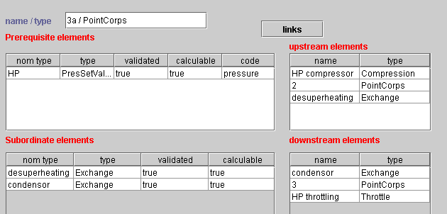
Thanks to this browser it is possible to easily navigate through the network which connects the different project elements, by simply double-clicking on any of the lines which are shown on the frame. It is thus possible to check the consistency of the system description and/or understand its logic.
Recalculating Multiple Selections
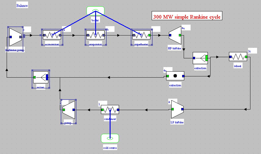
In version 1.5 and later, a special method is used to facilitate work on multiple component selections. It is accessible from the Special menu of the diagram editor.
When a multiple selection is done, it can be loaded in this screen by clicking on the button “Update the selection from the editor”.
The list of elements selected (points, processes, nodes, heat exchangers) appears in a table. The order of these components can be changed using the scroll buttons located in the lower right part of the screen, and elements can be deleted.
The list of elements selected (note: for the time being, the points are not selected when the file is re-read) can be saved in a file in the “res” directory. This list can be reloaded by clicking on the button “Load a multiple selection from a file”.
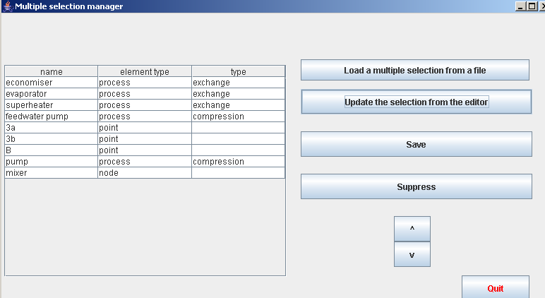
Once the selection has been made, various functions can be activated from the diagram editor:
- F5 launches an automatic recalculation in the simulator;
- F6 updates the multiple selection management screen by loading the current selection;
- F7 recalculates the different elements in the selection, in the order in which they appear on the multiple selection management screen. The values of the points selected will be updated if the values are displayed.
- F8 selectively displays or hides the values of the points on the multiple selection management screen. To display the values, type F6, then F3 twice (the first time selects all, and the second the multiple selection). Then, each time you recalculate using F7, the values displayed are updated.
These buttons are accessible from the Edit menu of the diagram editor:
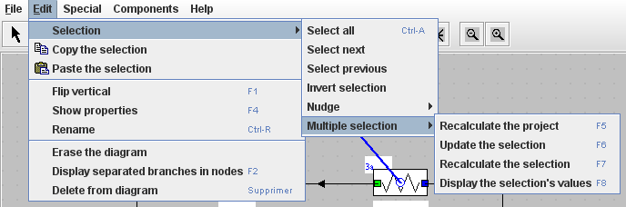
Pressure control
It is possible to define the pressure settings by associating a name and a value in the frame which can be displayed by double-clicking in the headband of the "Pressure settings" table located in the upper right part of the project frame (e.g. "HP", 165 for High Pressure and 165 bar):
Then, the points which must be at that pressure are connected with this pressure setting. This is done in the point frame by selecting "pressure controlled" and choosing "HP" from among the pressure setting list.
In the point screen, it is possible to define a pressure correction factor, by which the pressing setting value is multiplied to calculate the pressure. It is thus possible to automatically take into account pressure drops. In the example shown above, the pressure setting value is 165 bar ; as the correction factor is 0.98 (2% pressure drop), the point pressure is set to 161.7 bar.
When the pressure of a point is set in such a manner, we shall say that it is "externally set". Changing the values of the point pressures which are controlled by a given pressure setting is simply made by clicking on the "Set the pressure" button on the corresponding setting frame.
Heat Exchangers
For heat exchanger automatic recalculation, causality rules imply that the inlet temperatures and the mass flow-rates of the hot and cold fluid be known, and THERMOPTIM sets them from their processes (see the section on heat exchangers for more details).
Main project screen controls
The recalculation engine is controlled from the main project screen which displays the following information:
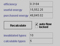
Above the "Recalculate" button and the "autoflow" checkbox are displayed three indicators whose sense must be recalled, as their labels may be misleading. Every process can be characterized, among others, by its "energy type", which can take three values : "useful", "purchased" or "other". The values which are displayed in the fields shown above are the following: "useful energy" is the absolute value of the algebraic sum of all Delta H values in the processes of the "useful" energy type. Similarly "purchased energy" is the algebraic sum of all Delta H values in the processes of the " purchased " energy type. Lastly, "effectiveness" is the ratio of the "useful energy" and the "purchased energy".
In general, this energy type is used to compute a classical thermodynamical cycle effectiveness. But it is also quite possible to use them to keep track of the sum of the enthalpies involved in two types of processes. You just have to characterize the corresponding processes as being either of the "useful" or the "purchased" energy type, the others being of the "other" type.
When you use the automatic recalculation engine, these values can thus be used as indicators of the recalculation process, as will be explained below.
The checkbox "locked" can be used to stop the automatic invalidation process when the system under investigation is comprised of loops.
Below the "Recalculate" button are shown the number of invalidated and calculable types. If you are interested in knowing which types are invalidated, this information is given in the link browser frames.
Automatic recalculation tools
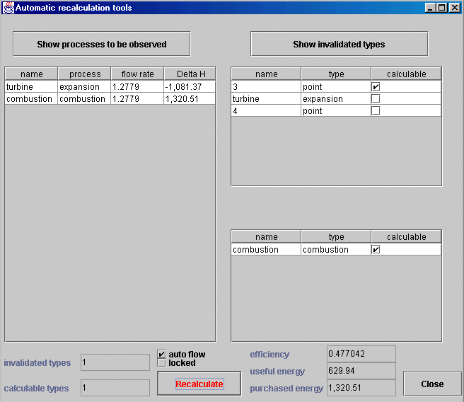
In order to facilitate the diagnosis of the model generated and the use of the automatic recalculation engine, a new window called "Automatic recalculation tools" has been introduced. It can be displayed from menu Special of the main project window, or by directly typing Ctrl R.
The concept of "observed" process allows one to better follow the calculation steps : a process is "observed" by selecting a checkbox located in the upper right part of its frame. In the automatic recalculation screen, all "observed" processes are listed in the upper left table, with their name, type, flow rate and enthalpy or internal energy involved. When the calculation is made, this table is updated, allowing one to follow the variations of these two key parameters.
Both tables in the right display invalidated and calculable elements for two successive recalculation steps: the last one appears in the lower part and the previous one above. Only the lower one is double-clickable, allowing one to display invalidated types. It is useful to follow the step by step invalidation propagation in order to check that recalculation is made adequately. Displaying the invalidated types is made either thanks to the corresponding button located in the upper right part of the screen, or automatically during the recalculation process. The recalculation engine can be activated from this screen or from the main project window.
The fields located in the lower part of the screen are the same as those dedicated to the recalculation engine in the main project frame.
Using the recalculation engine
Once a project is created or loaded, you should begin by calculating its different elements step by step, to make sure that all the necessary settings are appropriately selected.
You should also check the logical connections between the elements either by navigating from one type frame to those to which it is connected, or by using the Link browsers presented above, which give a comprehensive display of all the links.
If you want to use the automatic flow rate propagation, make sure that the "autoflow" checkbox is on, and that any process whose flow rate is set has its "set flow" checkbox on.
Once you have checked the connections between the elements, press the "Recalculate" button if the number of recalculable types is not null. Otherwise you have first to calculate an element connected at the inlet of the system in order to initialize the process.
When you click on the "Recalculate" button, the recalculation proceeds, the different calculable invalidated types being recalculated in turn, possibly in parallel. Obviously, as soon as a type is calculated, it invalidates all its subordinates and the process is iterative. When all the types which were initially calculable have been recalculated, the overall balance is made and the indicators updated.
Generally, new types have been invalidated. Iterate until the indicator values converge (generally 5 to 10 iterations are enough). I intend to automate this iteration later, but this is not done currently because the recalculation engine is still under development.
If the recalculation does not converge, there is most probably a problem in the interconnections or in the flow-rate propagation process: you may have to set the flow in a few processes by selecting "set flow" and entering an appropriate value.
If you select "locked" on the project screen, the invalidation process is locked, which means that when an element is recalculated, it remains validated, even if one of its prerequisite types becomes invalidated. Generally the invalidation process comes to an end in a few iterations. If you want to restart it, unlock the project if it is still locked, recalculate a type and iterate…
Sensitivity analyses
A specific frame allows one to make simple sensitivity analyses:
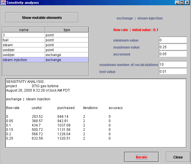
A table located in the upper left part allows one to display the three following types of elements and to modify the variables indicated between brackets:
- pressure settings (pressure)
- points without prerequisite (temperature)
- set flow rate processes (flow rate)
When you click button "Show mutable elements", the list of the corresponding elements of the project is displayed. To select one of them, double-click on its line, which opens its frame.
The type and the name of the element selected are displayed in blue in the upper right part of the sensitivity tool screen, and the name and the initial value of the variable appears just below.
The three fields located below allow you to define the minimum and maximum value as well as the increment to be used during the sensitivity analysis.
It should be noted that no consistency test is made on the sensitivity analysis parameter setting. The user should make sure that they are realistic.
Just below, two fields allow you to define the maximum number of recalculations and the accuracy requested. The accuracy test is made on the sum Delta of the absolute values of the differences between the useful and purchased energies obtained at two successive recalculation steps. If Delta is lower than the accuracy entered, the recalculation is stopped.
Once these parameters indicated, you start the sensitivity analysis by clicking the "Iterate" button. The results are summarized in the text field located in the central part, as a table giving the value of the variable, the useful and purchased energies, the number of iterations and the Delta value.
All these values are also written in file "sensi.txt" of sub-directory "res".
In this example, one has studied the influence of the steam injection flow rate on the output and efficiency of a steam injection gas turbine.
The above displayed example corresponds to the study of the influence of the steam injection flow rate on the behavior of a steam injection gas turbine.
The reasons which lead to the choice of the variables selected are the following: pressure settings (pressure), points without prerequisite (temperature), set flow rate processes (flow rate).
Pressure settings allow one to simultaneously make vary the pressure in a cycle part. A sensitivity study on these pressures is often requested.
Points without prerequisite will stay unchanged, except if the associated substance composition varies. To be able to make sensitivity analyses on their temperature may be interesting.
For the same reason, it is interesting to be able to modify the flow rate of set flow rate processes, which would otherwise not be modified.
Quick reference
The Quick Reference is a summary of Thermoptim manual giving basic information on the menus and the main concepts which are referred to in the software.
It is comprised of a frame containing tabs which can be selected by clicking on them. When you select one of the tabs, the corresponding information is displayed under the form of a short text.
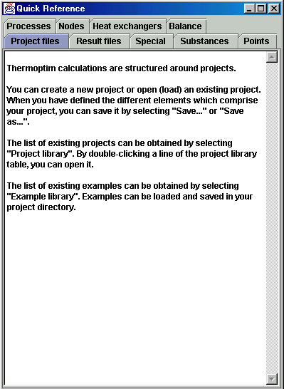
Interactive Charts
Presentation of the charts
Existing thermodynamic charts are presented in the form of paper abacus. Whatever care is taken by editors in the choice of color sets for distinguishing the various curves shown, it is always difficult to read them, and interpolation may lead to significant errors. THERMOPTIM interactive charts allow one, by a simple mouse click, to display all relevant thermodynamical properties of the fluid, providing thus a better accuracy and productivity gains.
Using the interactive charts is quite simple: position the crosshair cursor at the point whose thermodynamic properties you wish to get, and click so that they may be displayed on the screen. For the vapor charts these properties are: pressure (bar), temperature (K or °C), enthalpy (kJ/kg), entropy (kJ/kg/K), mass volume (m3/kg) and quality (dimensionless ratio of the mass of the gaseous phase to the total mass).
As the cursor positioning accuracy is a function of the screen resolution and is generally not very high, it is possible to make more precise calculations either by moving a target with the keyboard arrows, or by creating and editing points (named cycle points as a set of points usually represents a thermodynamical cycle).
THERMOPTIM interactive charts make use of a user friendly property editor to specify the input variables used when a point is calculated: the two first number columns from the left are considered by the software as designing the known state variables from which the other thermodynamic properties are calculated.
The different functions offered by the Interactive Charts are presented in details in their manuals or are presented in a Quick Reference frame which can be accessed to from the menu "Help".
Today, the following charts are available:
- vapor charts, which cover, either in temperature/entropy (T,s) or in enthalpy/pressure (h,p) coordinates, the liquid, liquid-vapor equilibrium and vapor zones, for fourteen pure substances, including steam.
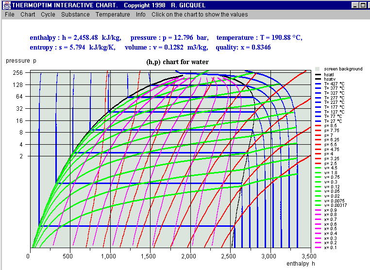
- psychrometric charts in which one can modify either the pressure or the dry gas composition (for air as well as pure or compound gases, such as combustion flue gases).
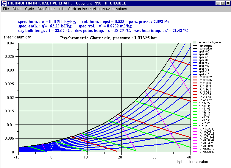
- Ideal gas temperature/entropy (T,s) or enthalpy/pressure (h,p) charts, similar to the vapor charts
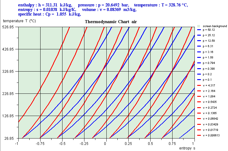
- external mixture charts that can represent a simplified mixture of vapors calculated by a thermodynamic properties server other than Thermoptim (see Volume 3 of the reference manual). The new charts are simplified compared to the others in that they show only the bubble and dew curves, as well as a single set of isovalues, i.e. the isobars for the entropy chart, and the isotherms for the (h, P) chart.
The preparation of the chart background can be made thanks to a special external class called CreateMixtureCharts.java which it is not necessary to present here.
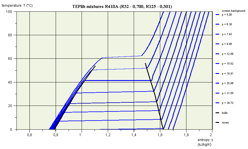
These charts being a variation of vapor charts, their use is explained in the documentation of these.
Connecting the simulator and the charts
The Interactive Charts can be either used independently of THERMOPTIM, or directly accessed in the software thanks to the following frame:
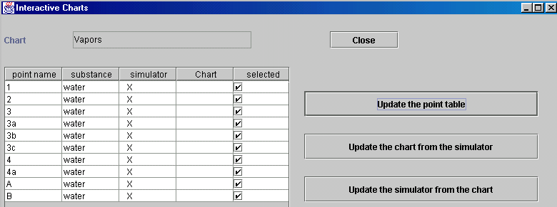
The Interface between the Simulator and the Interactive Chart frame is comprised of several fields and buttons and a main table showing the different points which either exist in the simulator or have been defined as cycle points in the chart.
The two first column show the names and the substance of the points. When a point is in the simulator, a "X" appears in the third column, and when it is part of the Chart cycle points, a "X" appears in the fourth one.
The last table column titled "selected" shows the point status: if a "X" appears, the point is selected for being taken into account in the transfers between the simulator and the charts, otherwise not. To change a point status, double-click on the corresponding line.
Above this table is the field indicating the chart selected. When you double-click on it, a combo-box presenting the different charts available is presented. The one you select is then displayed.
On the right of the table are three buttons:
- "Update the point table" browses through the project points and those which have been defined as cycle points in the chart, and lists them in the table, indicating the point substance and a "X" in the "simulator" and/or "chart" column depending on where the point comes from. In the example shown above, there are six points created in the simulator, and none in the chart.
- "Update the chart from the simulator" transfers selected point values from the simulator to the charts. Existing chart cycle points are updated and non existing ones are created. This button therefore enables one to plot on an interactive chart a cycle defined in the simulator. As the points are transferred in the order in which they have been created in the simulator, it may be necessary to reorder them to get a nice connected plot. This can be done thanks to the cycle point editor of the chart.
- "Update the simulator from the chart" transfers selected point values from the charts to the simulator. Existing project points are updated and non existing ones are created.
Dark coloring of the central isovalue
In the Demonstration and Education versions, the chart interactivity has been suppressed. In such conditions it is no more possible to know to which values correspond the various iso-curves which are displayed for temperature, enthalpy, quality…. In order to facilitate chart reading, the central curve (generally the fifth one), is now colored in dark, so that it can be easily identified. Deducing the other iso-curve values is then much easier.
Methodology for constructing and verifying models
Thanks to their powerful modeling environments, simulators like Thermoptim can be used to quickly design models of highly complex energy systems. Simulators can result in considerable productivity gains, provided that they are used wisely. Although they appear easy to use, there are a number of hidden traps that must be avoided.
To truly benefit from their potential, we must take a few precautions, or in other words, we must use the right methodology for constructing and verifying the models. The objective of this note is to provide Thermoptim users with advice based on past experience.
Think before starting to build the model
One of the most common errors made by first-time users is to start making their model before thinking through what they want to do. They open the software and start building a diagram without really knowing where they are going with it.
It is extremely important to start by having a good understanding of the problem at hand: What is the problem, what results are we looking for, what information do we already have, what information are we missing, what thermodynamic components must we use, what global architecture, what fluids are we working with, are there any state changes or chemical reactions (combustion, etc.), will the components of Thermoptim basic set be able to represent the fluid changes? At this point it is often necessary to reformulate or even transform the initial problem statement, and a sheet of paper or a whiteboard can come in handy.
Once the problem is defined, we can try to make it less complex by breaking it down into simpler parts, then rough out a solution using simplistic hypotheses to analyze each of the parts (perfect gas), and perform dimensional analyses, in order to get an idea of the orders of magnitudes of the flow rates and energy involved.
Build the model in several steps, and perform the calculations one by one
Only after this preliminary work can you begin to build the model in Thermoptim, if possible proceeding by iterations: resolve the sub-problems identified beforehand and check the consistency of the results for each one (especially the mass and energy balances), if necessary build external components, then assemble the full model and check for validity.
When building the model, we recommend saving the different versions of the project and diagram in separate files, to safeguard against data loss due to an input error, software error or computer error, and also so you can go back to a previous version if necessary.
It is also important to document the model as thoroughly as possible, both globally and in detail. In the different primitive types of Thermoptim, except the substances, there is a comment field where you can provide information on the meaning of a parameter setting, or the role of a point or a process. In the diagram editor, you can easily add text to distinguish the main groups of components representing the parts of the model. The documentation work is always easier to do when the model has just been built, rather than several months later. It’s also much easier to work with a documented model that provides information on the choices made than to try to remember why you did what you did at some later date.
Until your model has been checked (next step), it is better not to use the automatic recalculation engine, but rather to perform the calculations one by one, component after component, following the flow logic of the fluids used. In this way, you will not automatically spread errors that may skew all of your parameter settings.
Restart Thermoptim after building a complex model
Despite all precautions taken in developing the software, experience has shown that the simulator can behave oddly, especially when performing automatic recalculations, when you build a model for the first time. These problems disappear when you restart the program.
So get in the habit of saving your work, i.e. the project and diagram files, and then exit Thermoptim, whenever you create a new model, especially if you start from an existing model and add or delete components or if you rename a file. Re-open and reload your model. This will eliminate any problems that arise when working with a new model.
Renaming elements of an existing project
It can be very economical to start from an existing model and modify it, but certain precautions must be taken to avoid spending hours testing the new model. In particular, it is necessary to be very careful when renaming substances, points and components. We strongly recommend using the “Rename” function (Ctrl R) accessible from the substance manager (see below) for substances, and the diagram editor for the others, because it changes the name not only in the primitive type selected, but also in all those that are logically connected to it.
Test the model thoroughly before using it
If the model contains a large number of components, there are numerous possibilities for error:
- errors in representation of the global architecture
- errors in connection of the points to the processes
- errors in the logical or thermodynamic parameter settings of the components
Consequently it is necessary to thoroughly test the model by checking that its structure is correct and the results are consistent, specifically with the orders of magnitude identified during your initial reflections. Thermoptim already performs various checks during the input phase, and displays messages when it detects a problem, but there are many errors that only the model designer can identify.
To facilitate this difficult step, the software provides the user with various functions (Diagram/Simulator interface, substance manager, interactive charts) and also has diagnostic tools in the standard version, accessible from the Special menu from the main project window.
Identifying modeling errors
In order to identify differences between the diagram editor and the simulator, version 1.5 of the interface includes two red buttons that can be used to search for modeling errors, and to delete selected problems (last column checkbox checked).
Modeling errors include:
- elements of the simulator absent from the diagram editor
- elements of the diagram editor absent from the simulator
- unconnected points present in the simulator
- unused substances
These new functions are used like the others: click on the button “Search for errors” to display all of the potentially incorrect elements. Click on the button “Delete the errors” to delete only the selected elements.
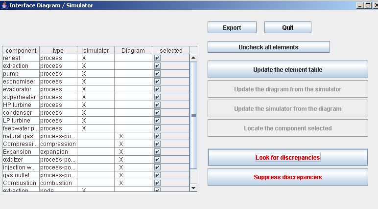
Once certain elements are deleted, new errors may appear, such as unconnected points that were previously connected or unused substances that were used before the points were deleted. It may be necessary to repeat the process in order to delete all of the errors.
To prevent unwanted operations, the simulator and diagram editor update buttons are disabled when you click on the search for errors button, and the delete errors button is disabled when you are using the interface in the usual mode.
Substance Manager
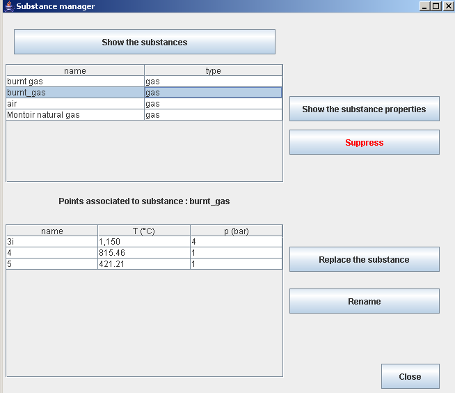
The Substance Manager, accessible from the Special menu of the simulator (except in the demo version) displays all of the substances used by the project. If you click on one of the lines, the points linked to this substance are displayed in the table below. This makes it easy to check the substances used in the projects and the points linked to them.
If a substance is not linked to any point, it can be deleted. If a line is selected and you click on “Display substance properties”, its composition is displayed if it is a gas, and its typical parameters are displayed if it is a vapor.
You can also replace a substance throughout the project, for example to test the effect of a substance change. For example, by considering the influence of Cp variation with temperature for ideal gases, you may obtain analytical results.
You can only rename a substance if it is not a vapor. Obviously, the new name must not be the name of a pure or protected gas or a vapor.
Interactive charts
Plotting a cycle on several interactive charts can be a very effective way to check the parameter settings of the different transformations involved: errors in pressures or temperatures show up as unusual plots, indicating a problem.
Diagnostic Tools
We recommend starting the tests by using these tools to check for point or process parameter errors that may have occurred if you inadvertently clicked in the wrong place. Look closely at the calculation modes (direct, reverse, open or closed system, etc.), the energy types that determine the balance, etc.
For the points, the search options are as follows:
- no prerequisite other than the substance that is associated to them or a pressure setting: theoretically, these points are never modified by the software, unless the composition of the associated substance changes or if the pressure setting is changed. They are initial parameters of a model.
- multiple prerequisites: if a point has more than one prerequisite, it means that it can be modified by more than one component. This is generally because, during modeling, it was incorrectly connected either to the outlet of two different processes, or to the outlet of one process and the inlet of the main process of a mixer. Additional explanations are provided below.
- calculated in open system with either p and T or p and h known.
- calculated in closed system with either v and T or v and u known;
- with a saturation pressure setting or a saturation temperature setting;
- not connected to a process: these points are not used and generally should be deleted. Note that when a process is deleted, the points are conserved to avoid losing their settings and so they can be used with other processes.
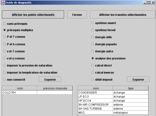
For the processes, the search options are as follows:
- open or closed system;
- type of energy: useful, purchased or other;
- pressure analysis: in Thermoptim, the pressures are initialized by default at 1 bar, then the user must set the values, since the software does it in only a very few cases. If the user forgets to do so or makes an error, convergence problems may appear. This search option covers on the one hand all of the processes other than compression, expansion and throttling in which the outlet pressure is greater than the input pressure (physical impossibility except for certain external processes), or is less than 80% of the inlet pressure (excessive pressure drop), and on the other hand all of the nodes through which the pressure increases (physical impossibility except for certain external nodes).
- direct or reverse calculation;
- set flow rate: this option facilitates checking of flow rate propagation consistency in complex projects.
For example, in the screen shot above, there is 1 point with multiple prerequisites, and the right part of the screen shows the result of a pressure analysis.
Point with multiple prerequisites
Double click on the line of the point “COLD RH” in the following figure to display its screen and access the links window.
The links browsers were created to analyze the logical links existing between the different elements of a project. They display four tables that show the links between a given type and the others. Access these tables by clicking on the “links” button of the primitive type.
The study of the prerequisite elements shows that “COLD RH” is defined both as an outlet point of the “HP TURBINE” turbine and as an inlet point of the main process of the mixer “FROM HP TURBINE & GAS…”, which is a modeling error that would have been difficult to detect without the diagnostic tool.
Pressure analysis:
There are six components in the pressure analyses that may have incorrect parameter settings. Double click on the table on the right to display their screens. For the first three, the outlet pressure was rounded up, and the error is negligible.
The next two components are external processes corresponding to a non-adiabatic compressor and a turbine, so it is perfectly normal for the pressure downstream of the first to be greater than the upstream pressure, and for the downstream pressure of the second to be less than 80% of its upstream pressure.
As for mixer “MIX2”, the pressure upstream of its main process is greater than the downstream pressure of its branches, which is clearly an error in parameter setting.
Thus, the diagnostic tool identified three negligible errors, two normal pressure changes in external processes, and one parameter setting error at the outlet of a mixer. Since the project involves sixty or so points and processes as well as fifteen or so nodes, identifying these errors would have been difficult without this tool.
Test the automatic recalculation
If everything looks good after these checks, save your model, then test it in automatic recalculation mode. As we said before, this step must not be performed too early, on a model that has not been tested as described above. However, an error-free model will be recalculated without difficulty, and the recalculation engine will perform various sensitivity analyses that are extremely valuable for judging the validity of the model.
If you want the flow rates to be propagated automatically, make sure that the option “auto flow rate” is selected, that the processes with preset flow rates are specified, and test the consistency of your model using the diagnostic tools.
Once you have checked the model thoroughly, open the recalculation tools screen and click on the “Recalculate” button if the number of calculable types is not zero. Otherwise, you first have to calculate an element located upstream of the system.
When you use the automatic recalculation engine, the calculable invalidated types are calculated as well, in parallel as the case may be. As soon as a type is calculated, it invalidates its subordinates, rendering the process iterative. When all the types that were initially calculable have been recalculated, the global balance is performed and the values of the indicators are updated. In most cases, new types have been invalidated. Iterate until the indicator values stabilize (5 to 10 iterations are usually enough).
If the processes do not converge, it is probably because there is a problem in the interconnections or the flow rate propagation: It may be necessary to set the flow rate of one of the processes, especially in the different loops.
In the Professional version, you can make the repeated recalculation automatic from the optimization method screen, with stop criteria based on the convergence of the model.
If you select the “locked” option, the invalidation system is disabled, which means that when an element is recalculated, it remains validated, even if one of its prerequisites is invalidated. This makes it possible to finish the recalculation process in just a few iterations.
If difficulties appear during the automatic recalculations, in most cases the thermodynamic parameter settings are incorrect, or the model itself must be revised.
Controlling the flow rate
In practice, it is very important to be able to control the flow rate. In Thermoptim, this control is performed by the nodes and the connections between processes.
In the mixers and the separators, the flow rate propagation is quite simple: in a mixer the flow rate of the main vein is the sum of all branch flow rates, and in a separator, it depends on the quality of the vapor entering the node and the drying effectiveness.
In a divider, the flow rate of the main vein is generally distributed among the different branches proportionally to their flow rate factors. There is one exception however: it is possible to set the flow rate in a process at the outlet of a divider, provided that this node has two branches, namely the one with the set flow rate and another one. In this case the flow rate of the second process is set equal to the flow rate of the main vein, minus that of the branch with the set flow rate, and the flow-rate factors are recalculated accordingly.
Flow rate can be automatically propagated between two processes when the following rules are met:
- First, the two processes must be directly connected. If the point connecting them is also connected to the third process, the problem becomes much more complex, and cannot be solved unless there is a diagram in which the valid connection is the only one (this issue is discussed in more detail later in the manual).
- Second, the automatic flow rate propagation system must be enabled by selecting the “autoflow” checkbox located next to the “recalculate’ button.
- Third, one may wish to simultaneously enable the automatic flow rate propagation in most processes and disable it in some of them. This is particularly useful when there are loops in the process networks. It can be done by checking or unchecking the "set flow" checkbox that appears in each process frame close to the "Delta H" field. When the "set flow" checkbox of a process is checked, its flow rate remains unchanged, except if it is connected to a node (except for the divider with a set flow mentioned above).