Thermoptim reference manual Volume 1
Table of contents
Copyright © R. GICQUEL 1997-2022 All rights reserved. This document may not be reproduced in whole or in part without the author’s express written permission, except for the personal licensee’s use and solely in accordance with the contractual terms indicated in the software license agreement.
Information in this document is subject to change without notice and does not represent a commitment on the part of the author
Foreword
Thermoptim documentation
Thermoptim documentation is comprised of several complementary parts:
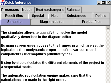
- a short documentation named Quick Reference available through menu Help: it gives access to tab frames introducing the main concepts used
- a printable documentation, mainly as pdf files
- on line e-learning modules with sound tracks named Diapason
- guided explorations of Thermoptim models
Printable documentation
The printable documentation is comprised of several parts which can be displayed through the Help menu of the simulator:
- Four Getting Started brochures allow one to quickly (less than half an hour) get used to Thermoptim. The first one presents an electricity steam cycle, the second one a combustion gas turbine, the third one a refrigeration cycle and the fourth one an air conditioning system
- The reference manual, itself comprised of three volumes and of the interactive charts manuals. The first volume introduces the software, the diagram editor, the use of the post-processing Excel macro and the optimization method, the second one deals with the simulator (screens of the different primitive types and advanced tools available in the modeling environment), and lastly the third volume explains how to use and build external classes
- a Frequently Asked Questions file is also available
Several examples with detailed explanations allow a user to get acquainted with the software thanks to a detailed presentation of how projects can be built. Three of the examples extend the Getting Started brochures.
The present document is the first volume of the reference manual. After a short introduction of the software, it presents the diagram editor and the optimization method.
Access the documentation via hypertext links
Windows versions 1.5 and later include hypertext links that provide direct access to the documentation and the FAQ. In order for the links to work, the file paths must be identical to what was entered in Thermoptim, otherwise they will not appear on the list.
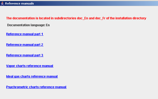
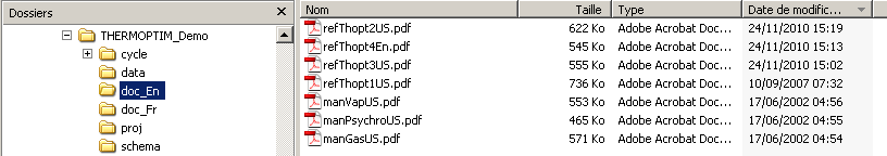
The documentation in English must therefore be structured as shown in the figure below. If you have an older installer, rename the files accordingly.
Diapason, online e-learning modules with audio
We have developed DIAPASON e-learning modules, which are online instructional modules with audio and animation allowing users to work on their own, at their own pace, with access at all times to oral explanations in addition to the written materials provided.
The following session is dedicated to being introduced to Thermoptim (in English):
https://direns.mines-paristech.fr/Sites/Thopt/en/co/session-s07en_init-first.html
There is also a special unit specifically on how to use and program external classes (in English):
https://direns.mines-paristech.fr/Sites/Thopt/en/co/session-s07en-ext.html
The purpose of these sessions is to introduce users to Thermoptim and enable them to become familiar with using it by building models using examples of simple energy systems (gas turbine, steam power plant, compression refrigeration system).
Guided explorations
In guided explorations of models built with Thermoptim, learners explore and parameterize models already built.
In Diapason sessions, learners learn how to build models on their own.
In , to reduce the difficulties associated with using the software package, they explore and parameterize models already built.
These guided explorations offer different activities to learners, such as finding values in the simulator's screens, resetting it to perform sensitivity analyses... Contextual explanations are given to them gradually.
Demonstration versions
All functions presented in the reference manual are not available in Thermoptim demonstration versions 2.5 and 2.82. In these versions the number of points and processes is limited to 10, the chart interactivity is disabled, as well as the advanced tools for diagnosis, automatic recalculation (including pressure settings), sensitivity studies and optimization. Furthermore only a subset of substances is available and all saving functions are disabled. It is however possible to read any Thermoptim project (whatever its size).
Version 2.82 is the one used in directed explorations.
The demo versions can be downloaded from this page.
Personalization of the workspace
The “Help” menu gives access to the global preferences screen, which enables you to personalize the software, except for the user interface language.
The language is selected automatically by Java, which loads the resources contained in the file “inth2.zip” present in the installation directory. To change the interface language, you must replace this file before opening Thermoptim.
From the global preferences screen you can define the working directories you want to use, select the online documentation language, as well as the various options presented below.
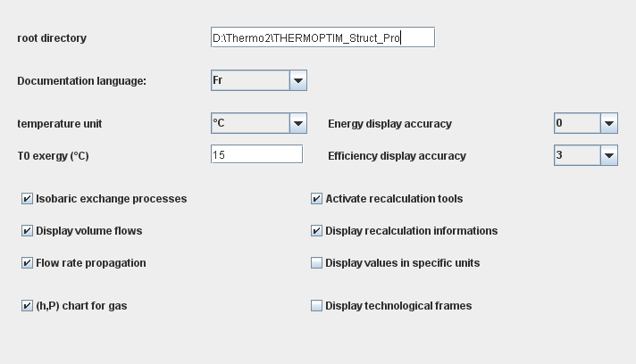
Global settings screen
Note: In general, the changes you make from the preferences screen are not implemented until you restart Thermoptim.
Working Directories
By default, Thermoptim uses a directory tree defined from the installation directory (root directory). A user’s working folders ("proj" for projects, "schema" for schemas, "cycle" and its sub-folders for diagram cycles, "pinch", "res") can be placed in another root directory, provided that this directory is indicated in the global preferences screen. The only rule is that the directory tree must be respected. The other files and folders specific to the applications, such as “data” and "documentation” must not be moved. In theory, the directory is changed immediately.
Temperature Units
In Thermoptim, temperature can be expressed in °C or in K. The temperature units are selected from this screen, but the change is not implemented until the application is restarted. You can also change the value of the reference temperature T0 used for calculating the exergy of the points.
Display Options
Documentation Language
In version 1.5 and later, you can consult the online documentation in French or English (if the translations are on line). The language is chosen from the global preferences screen, by selecting Fr or En for the documentation language.
Display Precision
In the energy balances, you can set the display precision of the energy values and the effectiveness. By default, the precision is set to 0 decimal for energies and capacities and 2 decimal places for effectiveness.
In the value input fields, you need to be able to enter a large number of decimal places, otherwise the calculation results would gradually drift if the calculation options were modified.
Automatic Recalculation, Flow Rate Propagation
You can disable the automatic flow rate propagation and the recalculation engine by deselecting the corresponding option in the global preferences screen. This can be useful from an instructional standpoint, to require the students to perform the calculations themselves instead of letting Thermoptim do it for them. By default, the automatic recalculation and flow rate propagation are enabled.
In order to simplify the display, in version 1.5 you can choose to show or hide certain fields, such as calculable or invalidated types (see section on the automatic recalculation engine).
By default, these fields are not displayed in the simulator. To display them, select the option “Display the recalculation information”.
Displaying Volumetric and Molar Flow Rates
In version 1.5 and later, you can also show or hide the volumetric and molar flow rates. To display them, select the option “Display the volumetric and molar flow rates”. Refer to the section on “exchange” processes in volume 2 for more information, specifically as regards set molar or volumetric flow rates.
Propagation of the Pressure in “Exchange” Processes
You can make the "exchange processes” isobaric if you wish. Select the option “Isobaric exchange processes” from this screen (by default it is not selected). When it is selected, the “exchange” process screen shows an isobaric option, which is selected by default when a process is created and saved as directed by the user. When this option is checked, the pressure of the upstream point is automatically propagated to the downstream point. Otherwise it is not.
Display in specific units
The external classes make it possible to model the thermodynamic evolutions that moist mixtures undergo. However, while the use for this type of calculations is to work in specific units (related to the dry gas flow), the default display mode does not allow this to be done in the software package, so the values displayed in the diagram editor can be confusing for users.
In order to give the possibility to change the reference system, an option allowing one to display flow rates in specific units has been added. For fluids that are not moist gases, nothing is changed, while for the others, the flow rate displayed is that of the dry gas, which is invariant, and the enthalpy H is replaced by the specific enthalpy q'.
Creation of (h, P) chart for gas
The option "(h, P) chart for gas" allows you to calculate and display ideal gas refrigeration charts, in addition to (T, s) entropy and (P, v) Clapeyron charts which are always built.
Internal Files
It may be helpful to know that every time Thermoptim starts up, it opens two temporary files placed in the installation directory, called "output.txt" and "error.txt". All of the internal messages generated by the application are saved in these text files. If an error occurs, the files generally contain valuable information on the cause of the problem (specifically missing files).
Security under Windows
Under Windows, the administrators generally prefer to install the software in protected directories in which the users cannot write files. Thermoptim writing certain files in a transparent way for the user, security access problems can exist.
The solution implemented consists in gathering in a particular directory all the files likely to be modified during the use of Thermoptim. This directory, of reasonable size (approximately 60 KB) can then be copied in a user directory distinct from that of installation. The address of this directory is stored in a file placed in the root of Thermoptim. At the time of the installation, the administrator writes, in the first line of a file called "Thopt.ini", the access path to a user writeable directory, and copies in this directory the file "thoptuser" containing on the one hand all the internal work files, which were until now in the sub-directory "data" except for "diag.ini", and on the other hand the user files (cycle, isoval, proj, res and schema).
The administrator then limits in reading and execution the access rights to the installation directory of Thermoptim, and authorizes the reading and the writing in the copy of "thoptuser". If "Thopt.ini" does not exist or contains an incorrect access path, Thermoptim continues to work like previously. If the user wishes to move his own working files, he copies in another directory file "thoptuser" and indicates its access path in the global properties screen. He must however always leave a copy of "thoptuser" at the place chosen by the administrator.
Security procedure under Windows
Unzip file "MAJ_NT.zip" containing the various files to be placed in the installation directory of Thermoptim. This file is in the "Special" file of this directory. It contains the Thopt.ini file initialized by defect with "." and the directory "thoptuser".
Move the file "thoptuser" in a user writeable directory, and enter between quotation marks the access path to this directory (for example, "D:\pub") with the first line of the Thopt.ini file, in the place of ".". Transfer in the sub-directories "proj" and "schema" from "thoptuser" your files describing projects and diagrams.
General presentation of Thermoptim
THERMOPTIM is applied thermodynamics software whose objective is to allow one to easily calculate complex thermodynamic cycles without making very simplistic hypotheses or without being involved in tedious calculations. It is based on the combination of a systemic analysis of the studied project, which allows to bring to the fore its main functional elements and their interconnections, and a steady-state thermal or thermodynamical analytical modeling of its various elements, necessary to calculate them.
The software is dedicated to both undergraduate students and professionals. The first ones are thus able to calculate realistic cycles without being hindered by the calculation difficulties which often discourage beginners. For the second ones THERMOPTIM furnishes a comfortable working environment which is currently missing. They are thus able to make more detailed analyses by investigating cycle options that they sometimes give up calculating for lack of an appropriate tool.
As compared to other existing software in this field, THERMOPTIM presents the following advantages:
- It includes the calculation of processes, nodes and heat exchangers, whereas most other tools only provide thermodynamic properties of fluids.
- Its primitive type set enables one to easily model a large variety of different thermodynamic systems, from simple cycles to complex utilities.
- Its graphical diagram editor provides a user-friendliness of particular interest for viewing large projects and controlling internal links.
- Thanks to its recalculation engine, it enables the user to automatically simulate complex processes and cycles.
Thermoptim four working environments
- The diagram editor allows one to graphically describe projects. It includes a palette comprised of any Thermoptim components; these can be displayed (process-points, heat exchanges, compressors, expansion devices, combustion chambers, throttling expansion valves, mixers, dividers, separators) on a working panel in which the components are located and connected by links. This graphical environment provides a user-friendliness of great interest for viewing large projects and controlling internal linkages. Furthermore, it allows for simpler data entry when creating a new project.
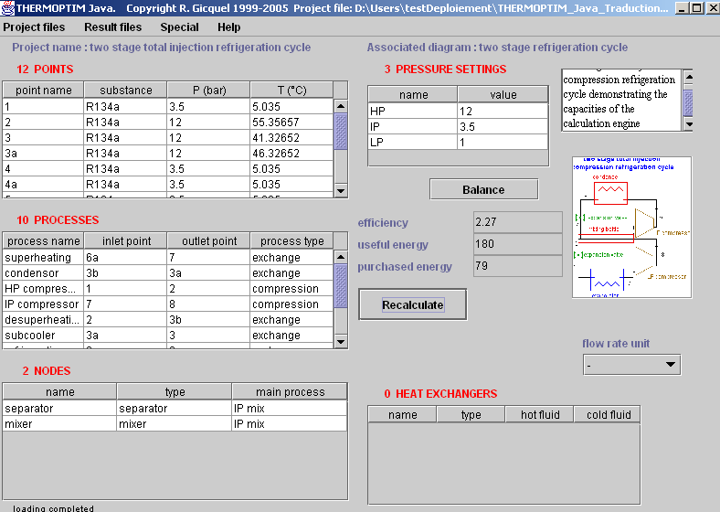
- The simulator allows one to quantify and solve the model described previously in the diagram editor. Its main screen gives access to the frames in which are set the logical and thermodynamic properties of the various model components (Thermoptim primitive types).
The simulator step by step calculates the different elements of the project. This is a sequential calculation mode differing from that used in other (matricial) modeling environments, in which the whole set of equations of the problem is solved at the same time. It is much easier to successively calculate the elements than to solve the whole system simultaneously. This way of doing however induces two difficulties: first it may be necessary to iterate several times to get the right solution when the project is comprised of loops, and second it may be difficult, for large and complex projects, to know in which order the calculations are to be done.
To solve the latter problem, a set of algorithms has been implemented. Named Thermoptim automatic recalculation engine, it represents a key element of the Java version of the software. A specific tool has been designed in order to follow the recalculation steps and thus be able to check the model consistency.
In addition, if a large project has been created, it may involve many elements such as points, processes and nodes. Using the diagram editor ensures that the connections between them are adequate, but not that their parameters are accurately set. A diagnosis tool has been developed to allow one to search and display the points or processes that share some characteristics, such as to be calculated in open or closed system, to have their flow rate set...
It is thus possible to selectively display the various model elements in order to check their settings.
Lastly the simulator allows one to make simple sensitivity analyses with regard to flow rates, pressures or temperatures.
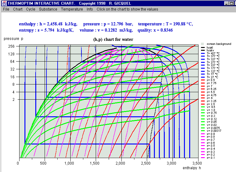
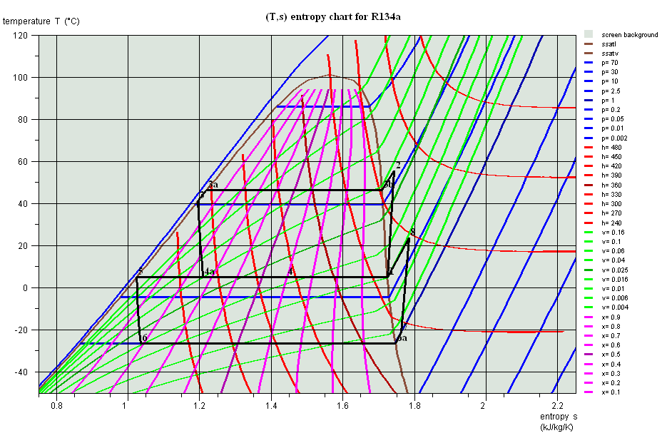
- THERMOPTIM interactive charts allow one, by a simple mouse click, to display all relevant thermodynamical properties of the fluid, providing thus a better accuracy. They can also be used to display thermodynamic cycles calculated by the simulator.
As of today, the following charts are available:
- Vapor charts, which cover, either in temperature/entropy (T,s) or in enthalpy/pressure (h,p) coordinates, the liquid, liquid-vapor equilibrium and vapor zones, for seventeen pure substances, including steam.
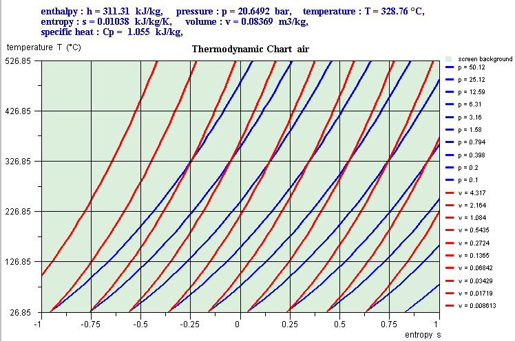
- Ideal gas temperature/entropy (T,s) charts in which one can modify the gas composition
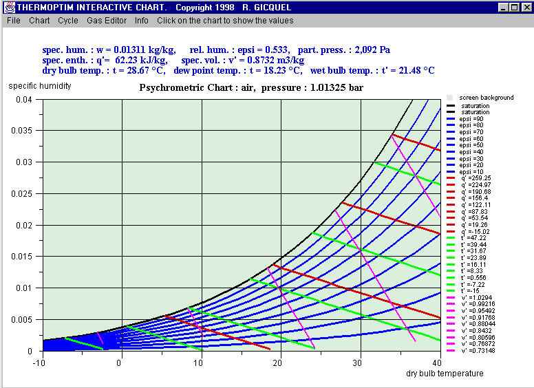
- Psychrometric charts in which one can modify either the pressure or the dry gas composition (for air as well as pure or compound gases, such as combustion flue gases).
- External mixture charts that can represent a simplified mixture of vapors calculated by a thermodynamic properties server other than Thermoptim (see Volume 3 of the reference manual). The new charts are simplified compared to the others in that they show only the bubble and dew curves, as well as a single set of isovalues, i.e. the isobars for the entropy chart, and the isotherms for the (h, P) chart.
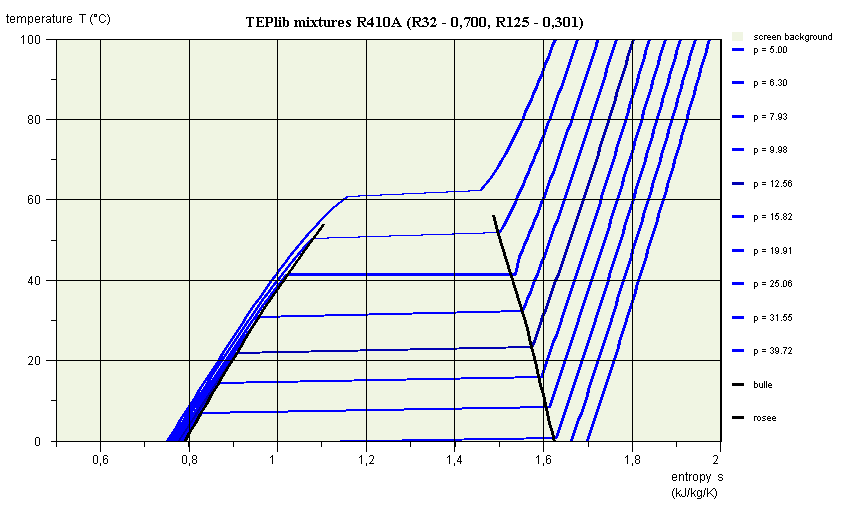
R410A entropy chart
The preparation of the chart background can be made thanks to a special external class called CreateMixtureCharts.java which it is not necessary to present here.
These charts being a variation of vapor charts, their use is explained in the documentation of these.
Thermoptim fourth working environment is its optimization method based on systemic integration, which is an extension for energy systems (electricity power plants, cogeneration units...) of the Pinch method developed for Process Engineering in order to optimize large heat exchanger networks such as those existing in refineries.
This method, by separating component irreversibilities from those which stem from the internal system configuration, allows to visualize in a physically meaningful manner the critical zones of the system and to highlight systemic irreversibilities which cannot be reduced. By putting in evidence pinches, it shows the zones whose design has to be subject to particular care, and thus constitutes a valuable guide where previously heuristic methods were employed, sometimes requiring numerous iterations.
In Thermoptim, these four environments are coupled by specific interfaces, the closest integration being realized on the one hand between the diagram editor and the simulator and on the other hand between the optimization tools and the simulator.
The main advantages of THERMOPTIM are the following:
- It provides a consistent modeling environment combining the inputs of systemic and analytical approaches. With a relatively small initial time investment, necessary to understand the underlying logic of the tool, itself rather natural and intuitive, it allows one to readily adopt a rigorous analysis method leading to sensible productivity gains. The models developed can easily be documented, saved and modified.
- Its basic component set enables one to easily model a large variety of different thermodynamic systems, from simple cycles to complex utilities. Very rapidly, the modeler is able to very easily represent an energy technology in a way which is at the same time close to reality and calculable by the software.
- The description of the problem is mad by using natural engineering concepts, the primitive types having a clear physical feel. The modeler can therefore concentrate on the physical analysis of the system because the mathematical and numerical translation of the model is created automatically by the software.
- The modeler does not write a single line of code, nor does he solve any equation, Thermoptim takes care of the coding of the project described. The user thus gets realistic results without any programming errors. If he or she wants to make calculations which are not included in the software, this is possible by using the output files provided, with a spreadsheet for example.
- The software is an open environment, written in the Java language. If need be, it is relatively easy to introduce new primitive types to represent components which are not yet available.
- As fluid properties are automatically calculated, the modeler can get very accurate results without being hindered neither by calculation difficulties nor by making unrealistic assumptions.
Principles of model building
Building the model of a thermodynamic system with Thermoptim is a very simple two step process:
- One starts by qualitatively describing the system graphically representing it as a set of components (more generally functionalities) connected together by links corresponding to fluid conduits and heat exchangers.
- Then one subsequently quantifies the model obtained by setting values of the parameters of the various basic types involved.
The diagram editor enables the user to undertake a qualitative design: at this stage the user enters a minimal amount of information requested to logically define the project (implicitly the types of the components selected on the palette, and explicitly their names, the outlet points and substances associated, as well as the flow rate involved). Subsequently, when a user connects these components together, key information is automatically transferred (for instance the inlet point of a component is set equal to the outlet point of the upstream component to which it is connected).
Once this phase is completed, it is possible to transfer the components to the simulator in order to instantiate the necessary primitive types, along with a default setting of their thermodynamic parameters. The model can then be quantified in detail with each simulator element being displayed easily by double-clicking either on the component in the diagram editor, or in a table within the main project frame.
Once the parameters are set and the elements calculated, the results obtained can be directly displayed in the diagram editor or in one of the interactive charts.
Thermoptim primitive types
THERMOPTIM allows one to calculate the complete state of different fluids (temperature, pressure, mass volume, enthalpy, internal energy, entropy, exergy and quality), for ideal gases and condensable vapors. These fluids can undergo various transformations or processes:
- Compression and expansion, in open or closed systems. These can be adiabatic or polytropic, and are characterized by their isentropic or polytropic efficiency.
- Combustion, also in a closed or open system, at set pressure, volume or temperature. Fuel can be introduced into the combustion chamber separately from the oxidizer, or premixed. The dissociation of the carbon dioxide can be taken into account.
- Heat exchanges with other fluids: the software is able to calculate the UA product or the overall heat transfer coefficient across the surface of a heat exchanger for the following configurations: counter flow, parallel flow, cross flow or (p-n) type. Once a heat exchanger is designed, it’s off design operation can also be determined.
- The software possesses a database of thermophysical properties of substances most commonly used in applied thermodynamics.
- throttling
Fluid networks are represented by nodes (mixers, dividers and separators), which conserve enthalpy and mass flow-rate. The other elements (compressors, turbines, combustion chambers, heat exchangers) can be easily connected into these networks.
Fluid mixtures can be made. These are considered to be ideal gases. Specifically, THERMOPTIM allows one to process water vapor / gas mixtures and provides six types of processes to study them (heating, cooling, humidification, supply conditions, desiccation).
The study of a thermodynamic system can be divided into five main tasks:
- 1) the analysis of the structure of the system under investigation, which identifies its main components and their connections: for instance, a thermal machine consists of heat exchangers, compressors, turbines or expansion devices, combustion chambers...
- 2) For each component, the identification of the thermodynamic fluids which are used: for instance, the fluid compressed in a gas turbine is air, which burns with a fuel in the combustion. The resulting flue gases expand in a turbine.
- 3) for each component, the selection of the kind of system to be considered (open or closed): for instance, the study of the compression in a piston compressor must be made in closed system, while that of the expansion in a gas turbine is to be made in open system.
Let us recall that a closed system (respectively an open system) is characterized by the absence (respectively the existence) of mass transfer through its boundaries.
- 4) The description of the processes which undergo the different fluids in the components, and the calculation of their evolutions in the components, taking into account their interconnections.
- 5) The calculation of the overall balance of the system analyzed.
THERMOPTIM focuses on the global behavior of thermodynamical systems, considering that the detailed internal design of components requires specific tools taking into account all sides of the problem (scientific bases, but also manufacturing and economical constraints). Fortunately, it is not necessary to have access to the detailed internal behavior of a component in order to be able to study how it fits inside a system. Generally, and this is true for most energy technologies, a component can be characterized by a small number of parameters and the values of its coupling variables. These parameters vary according to the type of component: a volumetric compressor is characterized by a volumetric compression ratio, a volumetric efficiency and an isentropic efficiency, a heat exchanger by an effectiveness and a number of transfer units… Coupling variables are pressures, temperatures, flow-rates…
The list of the main different functional elements which may be used for describing a thermodynamical system strictly corresponds to the concepts which are used in THERMOPTIM. We shall refer to it later as its set of primitive types. It includes the thermodynamic fluid properties, the points, the processes, the nodes and the heat exchangers described below, which are always grouped in a project.
THERMOPTIM has been designed in order to facilitate the calculation of complex thermodynamic systems, but it cannot replace the user for making the detailed analysis of the system under investigation, which corresponds to the three first steps above. Before entering his project in the software, the user must have made this analysis. Otherwise there is a risk that the description will be done improperly.
In this regard, the primitive type set used in THERMOPTIM constitutes a useful guide for modeling the system under consideration, and the software provides the user with analytical tools which allow him to check the interconnections by navigating between the different elements of the project.
THERMOPTIM makes use of three kinds of substances: pure ideal gases, composed ideal gases and condensable vapors (which are pure substances). Perfect gases are ideal gases whose specific heat is independent of the temperature. A given substance may exist (under different names) as an ideal gas and a condensable vapor. For instance, steam can be calculated as a vapor ("water") or an ideal gas ("H2O").
The substance can be pure, in which case its properties are predefined in the software, or it can be compound. In this case (that is possible only for a gas), the user has to define the composition from the other gases present in the database, by indicating for each of them, its name and its molar or mass fraction. Properties of the composed substance are then determined from those of its constituents.
A point designates a particle of a substance and allows the user to define intensive state variables: pressure, temperature, specific heat, enthalpy, entropy, internal energy, exergy, and quality. A point is identified by its name and the name of the associated substance. To calculate it, one may either:
- Enter the values of at least two state variables, generally its pressure and temperature for open systems, and its volume and temperature for closed systems.
- Automatically calculate them by using for instance one of the processes defined below.
Processes correspond to thermodynamic evolutions undergone by a substance between two states. A process associates therefore two points such as defined previously, an inlet and an outlet point. Moreover, it indicates the mass flow rate involved, and allows one therefore to calculate extensive state variables, and notably to determine the variation of energy involved in the course of the process.
Processes can be of several types: compression, expansion, combustion, throttling, heat exchange, and water vapor / gas mixtures (the latter includes six different categories of evolutions). According to each case, various characteristics of the process have to be specified, for example, in compression, its isentropic or polytropic efficiency, as well as the type of calculation which is required (open or closed system, direct or inverse calculation…).
A cycle can thus be described as a set of points connected by processes. To the extent that the mass flow rate fluid is the same in all the evolutions, processes and points are sufficient. If this is not the case, it may be necessary to describe at least partially the network of involved fluids. Then the first elements to define are the network nodes.
Nodes allow one to describe elements of the system where mixes and divisions of fluids take place. In a node, several junctions of fluid are connected to form a single vein.
If the node is a mixer, the various branches join to form a single vein. The mass flow rate of the main vein is equal to the sum of these of branches, and the enthalpy balance allows one to calculate the mass enthalpy and the temperature of the mixture.
If the node is a divider, the main vein divides into several branches, whose flow must of course be calculated. Its distribution between the branches is set proportional to the "flow-rate factors" specified by the user. The temperature and the mass enthalpy are of course conserved. The separator is a special divider which separates the liquid and vapor phases of fluid in the liquid vapor zone.
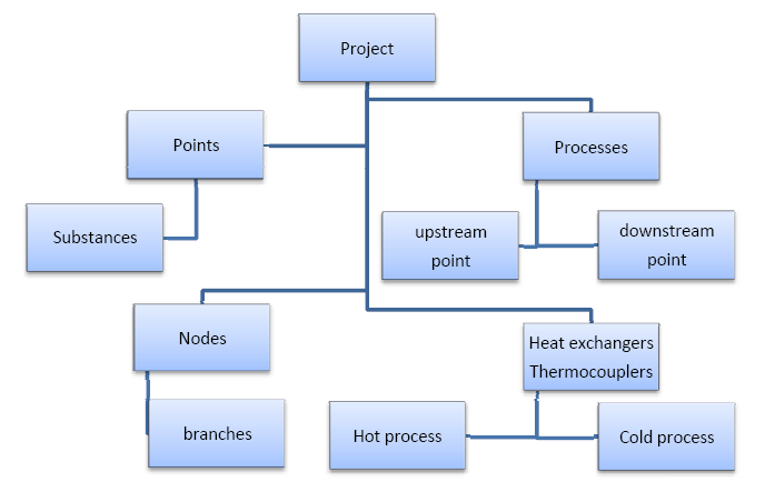
Thermoptim structure
One can mix several different fluids, provided that the mix is a gas. That means that if there are condensable vapors in the branches, one must make the hypothesis that they are in the gaseous state, and follow ideal gas behavior (this is why some substances exist at the same time as ideal gases and condensable vapors). Properties of the mix are calculated by application of the Dalton’s Law. The user has to verify that this hypothesis is valid. If this is not the case, results found by the software can be dissatisfactory.
The logical definition of a node is made by the association of processes, a process corresponding to the main vein (inlet process for a divider, outlet for a mixer), and n processes corresponding to branches. As the processes connect points, and each of these is linked to a substance, updates of flow rates and fluid states are made automatically by THERMOPTIM.
Thermal heat exchangers connect two fluids, one that gets hotter, and the other that gets colder. The simplest definition for a heat exchanger can be made with the identification of the two processes (fluids) that meet. The design of the heat exchanger can then be made if one indicates what constraints are set on the flow rates and temperatures (for instance minimum pinch, set value effectiveness).
Project storage and generation
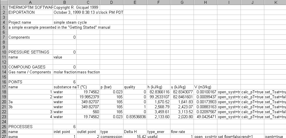
In order to facilitate the storage of projects during the development phase of Thermoptim-Java, the project files are saved under an ASCII format and read as text files.
All the information requested to create THERMOPTIM primitive types is included in this file. For instance, point 3b substance is water, its state is defined as follows: pressure is 165 bar, temperature 349.82 K, open system, p and T are known, the saturation temperature is set, the approach being 0…
This information consists of three different parts:
- the characteristics of the element, such as the isentropic efficiency of a compression
- the logical links between the element and the other primitive types, such as the substance for a point, the inlet and outlet points for a process
- the settings of the checkboxes which define how the calculations should be done, such as setting the saturation temperature, open or closed system…
Once this information is adequately entered, it can be used for complex tasks such as the automatic recalculation of the project. It must therefore be updated with great care when new elements are introduced or when the connections between them are modified.
One should note that THERMOPTIM makes use of two different kinds of ideal gases: protected ones and others. Protected gases are gases whose composition cannot be modified by the user, such as air.
They are stored in two different files: prot_gas.txt for the first ones, comp_gas.txt for the second ones for the English language, gaz_prot.txt and gaz_composes.txt for French.
The rationale for that distinction is to protect some gases from being inadvertently modified by a user who would have made a wrong connection such as selecting air as the outlet point substance of a combustion process… Therefore, it is possible to include in the protected gas file any gas whose composition must be kept unchanged. As this is not currently programmed in THERMOPTIM, the inclusion can easily be made with a spreadsheet software by copying the gas from the file comp_gas.txt to the file prot_gas.txt.
Project library management
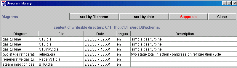
In order to facilitate project files management, a special frame allows to list in a table the different project files which exist in the user's project directory. To open it, select item "Project library" in menu "Project files". The table shows the project names, file names, dates of last modification, sizes and descriptions as they appear in the project comment. The list can be sorted by file name or date of last modification.
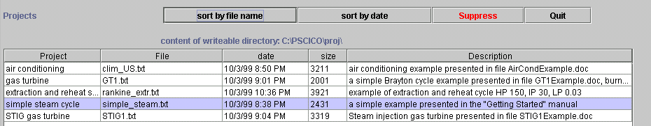
It is possible to suppress a project file by selecting it and clicking on red button "Suppress".
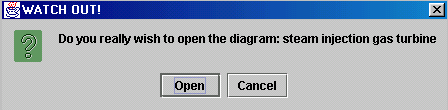
If you select a project and double-click on the selected line, a dialog indicating the name of the project selected and its description asks you if you want to open the project. If you accept, the project is loaded.
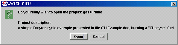
As you can see from this example, the description field in the table may not be large enough for the full project description to be listed. When you double-click on the project line, its description appears in full the dialog which is displayed.
It is also possible to display the list of examples which are available. To do that, select item "Example library" in menu "Project files" (here, the table has been sorted by date):
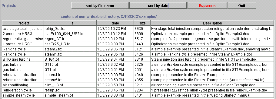
The only difference with the Project library is that the Example directory is non-writeable: you cannot suppress these files, nor modify them. If you try to do that, a message warns you that you are not allowed to do it. However, you may load one of the files and save it in your own directory, changing it as you wish.
Example catalog
You can load a catalog of projects and diagrams examples modeled with Thermoptim in order to facilitate their use in relation with a book.
It can be opened by line "Example catalog" of menu "Files", which displays a frame such as shown on the figure below. A structured list shows, for each of the book chapters, the references of the examples available, as they are given in the text.
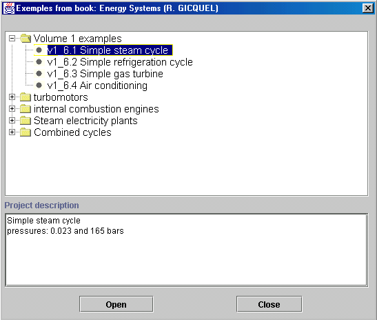
When one of them is selected, a short presentation of the example appears, enabling the user to check its selection. A click on "Open" makes Thermoptim load both the project and the diagram files if it exists.
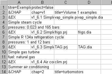
To build example catalogs, you just have to create a text file structured as shown on figure 6:
- The first line includes, on the right of "title=" the frame title, then a tab, and a code telling if the project and the diagram files directories are protected or not. If protect=false as on the figure, the user can directly save his or her modifications in these directories. If protect =true, the saving directories are those selected before. Indeed, this protection is only partial, as the user may choose to modify the example files, if he or she has the privileges to write in them, but he or she must do it deliberately, by selecting them through the "Save as..." menu lines.
- The second line, introducing a chapter, includes "&CHAP& followed by a tab, by "chap=" followed by the corresponding chapter ID, by a tab, and by the chapter title.
- Between two chapter lines are given series of examples, structured as follows: first characters "&EX" (to introduce an example), followed by a tab and the example reference in the book (beginning by the chapter ID), then a tab and the project file name, then a tab and the diagram file name. The following lines (until character "&" is met at the beginning) are the example description. Empty lines are not accepted, but a line with character " " is.
The end of a chapter corresponds either to a new one, or to characters "&FIN" indicating the end of the file. The relative path to the catalog directory and the catalog file name must be written between quotes in file "Loadlib.ini" located in Thermoptim installation directory or in "thoptuser" directory if the secure Windows NT setup is on. If file "Loadlib.ini" does not exist, the "Example catalog" menu line is disabled. The following lines are an example of file "Loadlib.ini" content:
"..\\ExLib"
"SystEner_RG.cfg"
Directories "proj" and "schema" containing the project and diagram files for the examples must be located in the catalog directory (here ExLib).
Using the Thermoptim diagram editor
Thermoptim is equipped with a diagram editor which allows one to graphically describe projects. This environment provides a user-friendliness of particular interest for viewing large projects and controlling internal links. Furthermore it allows for a simpler data entry when creating a new project.
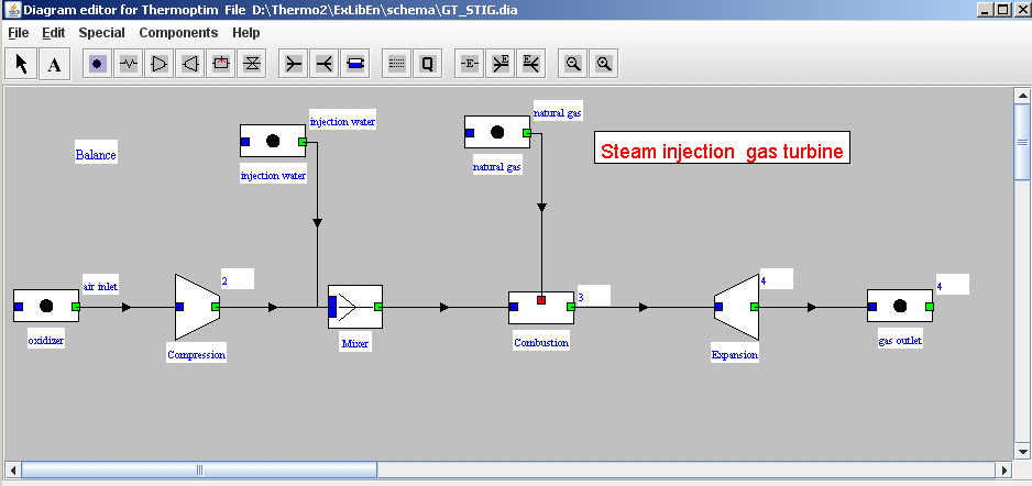
Presentation of the editor
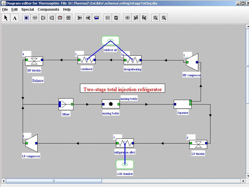
The editor looks like shown above. To open it, select item "Diagram editor" in menu "Special" of the main project window. It includes a menu bar with three menus, a palette comprised of Thermoptim components which can be displayed (process-points, heat exchanges, compressors, expansion devices, combustion chambers, throttling expansion valves, mixers, dividers, separators), and a working panel on which these components are placed and connected by links.
Since version 2.51, two icons to zoom the diagram in or out are shown on the right side of the palette. It is possible to enlarge or reduce the diagram to adjust its appearance on screen and when printed.
Graphical component properties
Property editor
The diagram component properties allow one to define but the minimum for creating a Thermoptim project, the detailed characteristics of the various primitive types being subsequently entered through Thermoptim regular screens. It is therefore necessary to have two saving files: the diagram description file and the usual project file.
The diagram component properties are thus mainly the names of the component, points and substances corresponding to the connections between the ports as well as the value of the flow-rate.
More precisely, it is generally sufficient to define the component by its name, and for its outlet port, the name of the point and the corresponding substance as well as the value of the flow-rate through this port. The inlet port properties are subsequently automatically updated when an upstream component is connected. If in addition the component does not introduce a new substance, the outlet port substance is also updated. The properties are mainly accessed to, either through a tab editor, from the Edition menu, or by typing F4.
Placement of a component
In order to place a component in the editor, select it on the palette by clicking on it, then direct the crosshair cursor at the chosen location, and click. The property editor is automatically opened. For all processes but process-points, it looks as follows:
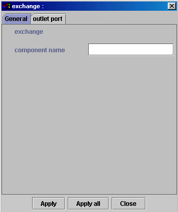
Name the component, then click on the tab "outlet port", and enter the point name. To enter the substance name, you may either type it if you know it, or get it from the list of available substances which can be displayed by double-clicking in the substance name field. Finally enter the flow-rate value, and then click on "Apply all" to directly validate all the tabs and exit the editor.
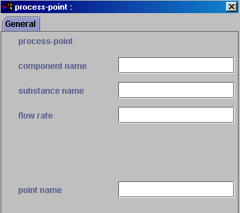
The number of tabs depends on the component selected. For Thermoptim nodes, the name is sufficient, the other properties being defined by the connections. For process-points, there is but one tab, to enter its name and that of the point as well as the substance and the flow-rate. If the point name field is empty, the point's name is that of the process.
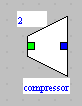
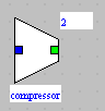
Once you exit the property editor, the component is displayed with its name below it and that of the outlet point above on the right.
By default, all components are oriented from the left to the right, but it is possible to orient them from the right to the left by selecting item "flip vertical" of menu Edition or typing F1:
The name of the outlet point is then displayed above on the left. If you flip it again, the component is oriented as initially.
Once the component is created, you have access to all its properties by selecting item "Show properties" of menu View. All the available tabs for this component are then available, including those which have been automatically updated during connections.
Inputting the flow rate from the diagram editor
To avoid confusion, in version 1.5 and later, you can set the flow rate from components in the diagram editor only when the component has been created, and not when it already exists. This is because once the simulator parameters are set, it is generally the simulator that calculates the flow rates, and there may be a conflict between the values entered in the diagram editor.
Comments
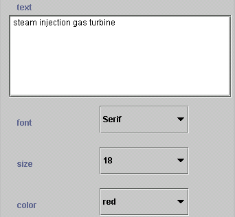
It is also possible to include comments and to choose their font, color and size.
To do this select the text component (image "A") at the left of the palette, and place it where you wish the comment to appear. The property editor allows you to enter the text and choose its font, color and size.
To modify the text, you can either do it by double-clicking in the left of the component (in the blue rectangle), or through the property editor (F4 or item Show properties of menu Edition). Note that tabs, line feeds and carriage returns are replaced by spaces when the diagram is saved (otherwise the saving file would not be of the right format).
External Components
Specific icons were added to represent the external components (

for processes,

for mixers, and

for dividers). The external component is then selected when the simulator is updated from the diagram. Volume 3 explains how to create and use these components.
Balance
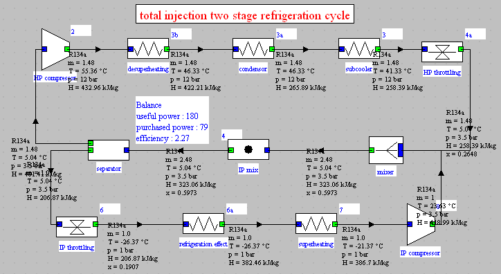
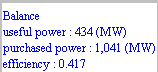
In order to be able to directly display on a diagram the overall balance of a cycle, a new component has been introduced (figure 1). Taken into account its specificity, it is not placed on the palette and can only be accessed from menu "Components".
It displays the values of the useful and purchased types of energy as well as that of the effectiveness; it is updated when "Show values" is selected. It can be used with or without the display of the point state values.
External source
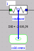
A new component has been defined to represent the thermal exchanges between a system and the environment. It is a passive component named "external source", which can be connected to exchange processes or to other external sources. This component's symbol on the palette is

, as it represents a heat exchange at the system boundaries. A given external source can be linked to several processes. When the point state values are displayed on the diagram editor, the enthalpies involved in the various processes connected to an external source are shown.
By default, the link between an external source and an exchange process is not named, but it is possible to rename it (line "Rename" of the "Edition" menu, or Ctrl R). If there is a multiple link with an external source there can be but a single name.
Connecting components
You can create links of two different types:
- The first one corresponds to pipes connecting components, through which flow thermodynamic fluids. Their orientation is marked by an arrow.
Each component is equipped with small colored rectangles which are connection ports between which links can be set. Inlet ports are colored in blue (or red for the fuel of a combustion chamber), and outlet ones are green. The small rectangles (in practice squares) allow to graphically set up but one graphical connection (however several can be set programmatically), whereas the large ones, used for mixers and dividers, allow to make multiple connections.
To connect two components, click on an outlet port (green) and drag the mouse to an available inlet port (blue), and then release the button. If the connection is allowed a link is created.
Since two nodes cannot be connected to each other, nor a node with the oxidizer or fuel of a combustion chamber, this constraint is circumvented by inserting a process-point between them.
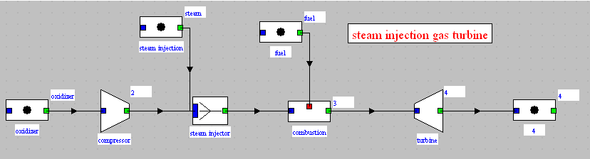
For instance, the previous diagram shows different such links: the process-point "oxidizer" is connected to the compressor by a single link, while the mixer has two input links, coming from the compressor and from process-point "steam injection".
- The second type of link is used to represent heat exchangers. It is not oriented and connects two "exchange" components. In this manual, we shall talk of exchanger connection to refer to this type of link.
An "exchange" component has in its center a small maskable exchanger connection port, which appears (as a small blue or red circle) only when the mouse is located above it, or when it is connected with another such component to represent a heat exchanger.
To make the connection, click on this port of one component and drag the mouse to the same port of another component and then release the button. During the connection the name of the exchanger is asked for. The port is blue for the cold fluid and red for the hot one.
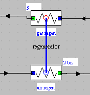
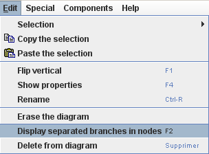
Branches display in nodes
The branches of the nodes can be viewed in two ways: either by default, all being superimposed, or being separated. To change the display mode, hit the F2 key or select the line “Display joint branches in nodes” in the "Edit" menu. The figure below shows the appearance of a diagram when the branches are shown separately.
Refining the positioning of components
It is possible to refine the positioning of the components selected using the small arrows on the keyboard and holding down the shift key. Each time an arrow is hit, the affected components move slightly in the chosen direction.
Deleting one or more components
To delete one or several components, select them, then select item "Delete from diagram" of menu Edition, or click the "Delete" key.
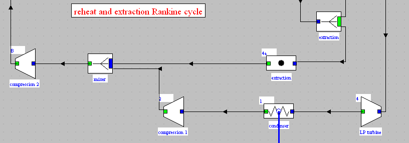
Duplicating one or more components
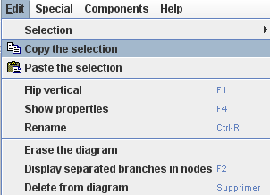
It is possible to duplicate one or more components of the diagram editor using the Copy / Paste functions from the Edit menu, with the exception of text blocks and the balance sheet component. The links are not duplicated either.
"Copy selection" copies all the components.
"Paste Selection" allows you to duplicate the selection, according to the following rules.
The names of the components must be different from the original, but those of their inlet and outlet points, if any, can optionally be retained. That's why Thermoptim first asks you if you want to change them or not.
It then asks you to set the suffix which is added to the existing names to be modified, the default value being "_copy." Enter the suffix that you want. The components are created and positioned on the diagram editor, slightly offset from the originals.
Of course, the names of the substances are not changed.
Once components duplicated, you can link them and transfer them into the simulator as explained below. Note that the points can also be duplicated one by one, from their screen.
Renaming components
To rename a component, select it, then select item "Rename" of menu Edition, and enter the new name. Both the component in the diagram and the corresponding Thermoptim element will be renamed
Diagram saving
As indicated above, the project and the diagram are saved in two different files. By default, the latter is saved in sub-directory "schema". For the time being, synchronization between the names of both files is not automatically made. It may therefore be advised to save the projects and diagrams with the same name, and extension .prj for the first ones, and .dia for the latter.
Diagram library management
In order to facilitate diagram files management, a special frame allows to list in a table the different diagram files which exist in the user's "schema" directory. To open it, select item "Diagram library" in menu "File". The table shows the diagram names, file names, dates of last modification, sizes and descriptions as they appear in the project comment. The list can be sorted by file name or date of last modification.
It is possible to suppress a diagram file by selecting it and clicking on red button "Suppress".
If you select a diagram and double-click on the selected line, a dialog indicating the name of the project selected and its description asks you if you want to open the project. If you accept, the project is loaded.
Links between the Simulator and the diagrams
The links between the simulator and the diagrams can be made either directly through the editor, by double-clicking on an enough defined existing component, or through a specific interface.
In both cases, the elements to be transferred are updated in the other environment, those not concerned by the transfer being unchanged. Thus, if some points or links are no more useful, they are not deleted.
Creation of a diagram from the simulator
The Diagram / Simulator interface allows one, as the one which is used to transfer points between the interactive charts and the simulator, to create a diagram from the simulator. It can be accessed to from menu Edition.
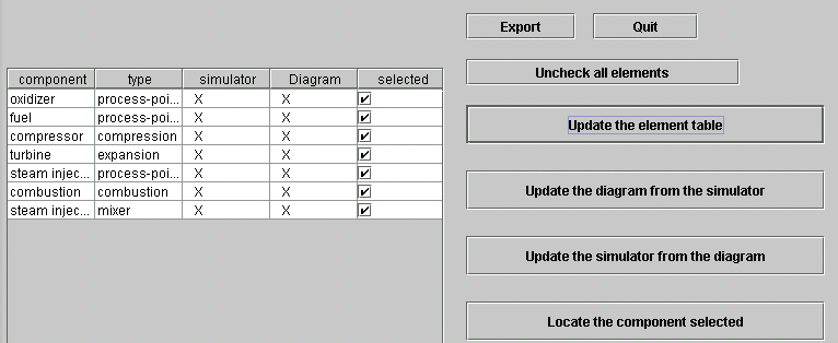
The list of transferable elements is displayed in a table, and the user can select those he wishes to create or update. Their location is defined by the last rectangle selected in the editor. It is thus possible to progressively transfer elements at various locations of the diagram by choosing the destination zone on the working panel.
By default, all the elements are selected when the list is updated, but a button allows one to deselect all of them for a progressive transfer.
The links between the components are made on the basis of the points shared by the processes, and of existing connections for the mixers, dividers and separators.
The diagram is created as follows:
- During a first phase, the components are created if they do not already exist, and those corresponding to processes are initialized (names of points, substances, flow-rates...) (for mixers, dividers and separators, there is no need for an initialization, their definition being made when the links are set up).
- During a second phase, the links are created. For the processes, a link is created each time a point is shared by two diagram components. When a given point is used by several processes, it is therefore possible that multiples links be created. It is then up to the user to delete by hand those which have no physical meaning, as this operation cannot be automated. For mixers, dividers and separators, the connections are made in two steps: creation of the link with the main process, then of those with the branches. For separators, the upper outlet port is used for the vapor, the lower one for the liquid (more dense).
- When a heat exchanger exists in the simulator, both exchange components are linked by an exchanger connection named after the heat exchanger if both components exist and if at least one of them is selected.
The button Export allows one to write in file "output.txt" the list of the elements displayed in the window, with the following code: "1" for "yes", and "0" for "no".
The button "Locate the component selected" allows one to move the visible part of the diagram so that the component selected in the left table may appear on the screen. This function is useful for large projects.
Looking for discrepancies
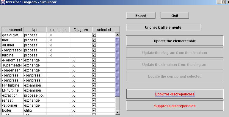
Interface Diagram / Simulator of version 1.5
Updating a substance from the diagram editor
It is now possible to change a substance from the property editor of a component in the diagram editor. Both the inlet and outlet points of the simulator have their substance modified when one double-clicks on the component or when one transfers it in the simulator from the Diagram editor / Simulator interface.
Creation and update of the simulator elements
The creation of the simulator elements is done either directly by double-clicking on one of the components, either from the Diagram / Simulator interface. In order for the operation to be possible, the component must be enough defined, which means that its name and those of its ports points and substances must have been defined.
Otherwise, the component is colored in yellow, so that it can easily be identified. Show then its properties, and enter the missing values, and try again to create the simulator element.
Once the types are created, their characteristics must be entered in the regular simulator screens, and saved in a usual project file. When an element already exists, e.g. when exists in the simulator an element of the same name and the same type, a double-click on the component displays it.
The structure modifications (addition of new components, connection changes...) made in the diagram editor are transferred in the simulator when one double-clicks on a component or makes an update from the Diagram / Simulator interface.
Generally speaking, it therefore appears preferable to make all structure modifications from the diagram editor, and to set the simulator element characteristics by displaying them from their graphical component. This way one takes full advantage of the visual interface, and one avoids on the one hand placement problems occurring with components created from the simulator, and on the other hand the automatic creation of physically meaningless links if some points are shared by several processes, as it is often the case for complex systems.
Connections between two nodes
As it is impossible to directly connect two nodes, a process-point is automatically inserted between them if you try to do so. You then just have to set its parameters.
Note concerning process-points
The case of process-points merits further discussion. These processes are in particular useful when one creates large projects. They allow one to define fluid inputs or outputs, to connect nodes…
As for the simulator a process-point is an "exchange" process whose inlet and outlet points are the same and whose name is the same as that of these points, it is only when these conditions are met that a diagram editor component of the type "process-point" is created from the simulator.
One of the problems is that a process-point may lose this particularity when a project is modified. For instance when another process is connected to it, it becomes a simple "exchange" process. As long as these modifications are made from the editor, there is no problem, but if one wants to update the editor from the simulator, a new "exchange" process may be created, with the same name as the initial process-point. In this case, one should delete the latter component, which is useless.
Viewing the simulator results on the diagram editor
You can directly view the point state values on the diagram, by selecting item "Show values" in menu Special. This enables you to have a comprehensive view of a whole project.
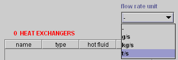
Choosing the flow rate unit
Introducing flow rate and power units
In version 1.5 you can choose the flow rate units from a drop-down menu located in the lower right of the simulator screen.
Once you have chosen the flow rate unit, the power unit can be displayed in the balance of the diagram editor, as well as in the process screen.
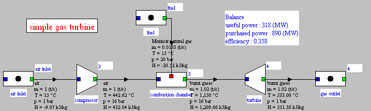
Diagram of a gas turbine
The flow rate unit selected is saved in the project file.

Working panel
Dimensions of the working panel
The diagram editor working panel dimensions are by default a 2000 pixel width, and a 1000 pixel height. For large projects, it may be necessary to increase it, which can be done by selecting item "Dimensions of the working panel" of menu "View". The following frame is opened. You just have to enter the desired values and to validate. These values are saved in the diagram saving file.

Printing a diagram
You can print a diagram by selecting item "Print" of menu "File". When the diagram size exceeds the size of the paper from the printer, the easiest way is to use the zoom out button to reduce the size of the diagram until it fits within the sheet.
Two other possibilities exist for resizing the diagram:
- Either, if the printer allows you to resize the printing, to choose the landscape format, select the paper size requested, then resize by a factor to be chosen by trials and errors.
- Or start by printing the diagram in a Postscript ".eps" format (many printers propose this option), choosing the landscape format, and possibly resizing. Once the file created, it can be inserted as an image in a PowerPoint or Excel file, the simpler being a PowerPoint slide. On your screen you will see nothing but a few text lines, which is normal.
You then just have to print the page or the slide where the image has been inserted, indicating that the printing has to be resized to match the sheet size. Usually this latter solution gives the best results.
Using the Excel post-processing macro
For a single Thermoptim diagram file, there are numerous possible project files corresponding to different parameters settings for the model. In the Standard version and higher, there is a function enabling you to perform sensitivity studies, but it can keep track of only a small number of parameters.
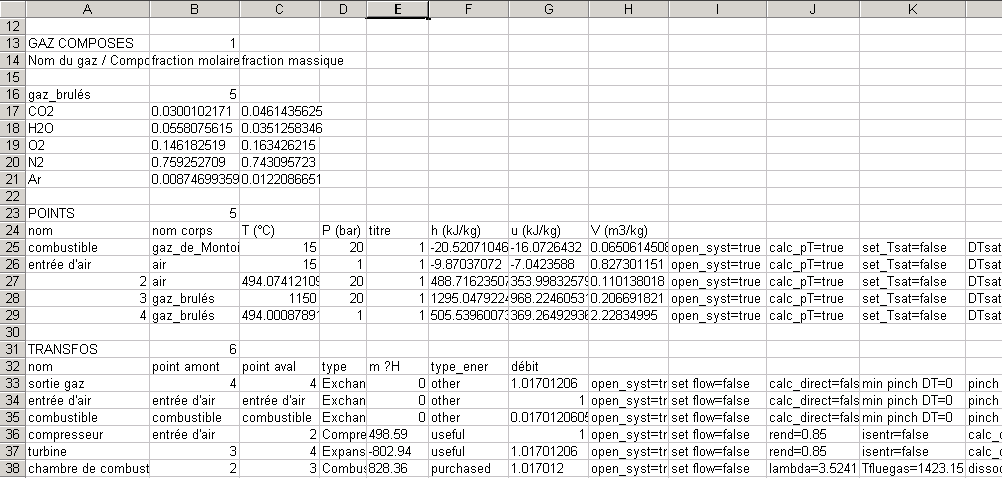
Screen shot of a Thermoptim project file
Let us look at the structure of the Thermoptim project files (figure below). The parameter settings are placed in text fields separated by tabs, so each appears in a specific cell if the file is opened in a spreadsheet program. As you can see in the figure below, each cell contains either a value (the enthalpies of the points are given in column F, from line 25 to 29), or an “identifier=value” pair (like cells J38 and K38, which give the air factor and the combustion temperature of the combustion chamber).
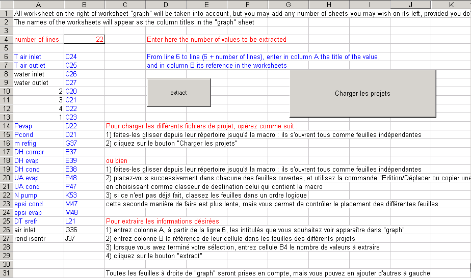
Worksheet where the cells to be extracted are defined
With the Excel file MacroPostTraitementRef.xls located in the “special” menu of the installation directory, you can readily post-process a group of similar project files relating to a single model. This file has two macros that enable you to load the project files, and then extract selected values. These can be simple values or “identifier=value” pairs. Below are instructions on how to use the macros.
Start by closing all open windows in Excel, then open the spreadsheet MacroPostTraitement.xls and click on the left-most worksheet called “macro”. In the example below, the print area in the macro worksheet is lines 4 to 10. The rest are explanations on how to use the macro, in French and English.
There are two steps involved:
- First, you load the different project files in the spreadsheet program,
- Then you define the values to be extracted and run the extraction macro.
Loading the project files in the spreadsheet
- Open the file explorer in your operating system (Windows in this example) and place the window just above the MacroPostTraitement.xls spreadsheet.
- Select the files you want to process;
- Drag them to the MacroPostTraitement.xls spreadsheet; They will each open as separate worksheets;
- In each file, click on Edit/Move or copy a worksheet" and choose MacroPostTraitement.xls as the destination spreadsheet. Make sure you place them to the right of the worksheet called “graph”.
- Arrange the worksheets in a logical order, if necessary.
You can also replace steps 4 and 5, which can be time-consuming when there are a lot of worksheets to load, by clicking on the button “load the projects”, which will automatically load the projects. However, you will not be able to change the order in which the worksheets are arranged.
The project files thus automatically appear as worksheets in the spreadsheet, identified by their name without the extension. In this example, we are assuming that there were no worksheets to the right of the "graph" worksheet. You should delete any worksheets relating to another project.
Defining the values to be extracted and running the macro
To extract the desired information:
- In column A, starting at line 6, enter the labels you want included in the post-processing worksheet “graph”;
- In column B, enter the cell reference in the project worksheets;
- When you have finished, enter the number of values to be extracted in cell B4 (outlined);
- Click on the button "extract".
In the example above, we wanted to extract the energies used in three processes (the compressor work, the turbine work, and the heat released in the combustion chamber in cells E36 to E38, see the figure showing the project file), as well as the temperature of points 2 and 4 (compressor and turbine outlets, cells C27 and C29, see the figure). As there are 5 values to be extracted, we enter 5 in cell B4.
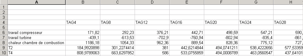
Values extracted by the macro
Once the values to be extracted are selected, run the macro by clicking on the "extract" button. The macro runs through all the worksheets located to the right of the worksheet “graph” and copies the values of the selected cells, building the table shown in the figure below.
Note: We recommend configuring your machine so that the decimal separator is the period and not a comma, by selecting English as the regional option. Otherwise errors may occur in reading the values.
Each line corresponds to one of the values selected, and each column corresponds to one of the worksheets.
Post-processing
Once the values are extracted, you can access the normal features of Excel, for post-processing.
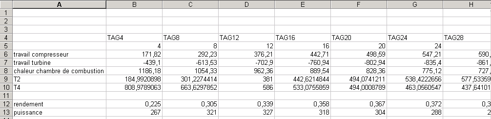
Specifically, on line 5 or lower, you can enter the value of the parameter that has been modified from one project file to another (the macro has no way to determine this automatically). In this case, it was the compression ratio, concatenated to the character string “TAG” in the file name.
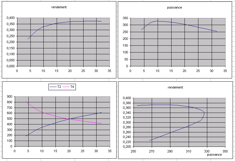
You can easily recalculate the machine’s effectiveness and power values based on the extracted values, and plot the evolutions of all of these parameters as a function of the compression ratio, or for example, the evolution of the effectiveness as a function of the power (figures below).
Post-processing
Optimization tools
Basic Concepts
If you disregard the relatively complex theory that this method is based on (derived from the pinch method with a distinction between component irreversibilities and system irreversibilities - see references), Thermoptim optimization method is relatively easy to present and use.
Let us start by saying that this is a variant of the Linnhoff method applied to energy systems. The Linnhoff method is used when designing complex exchanger system with a great many streams, for chemical engineering applications for example.
A relatively complex energy system can have quite a large number of streams that exchange heat, some getting heated, some cooled. These streams are generally matched in a number of different ways, and selecting the best architecture is not necessarily intuitive, far from it. However, this architecture has a direct effect on internal irreversibilities, and thus on the system’s effectiveness. By maximizing the internal regeneration, we obtain the best performance.
To choose a powerful exchanger configuration, thermal integration methods appear to be the best. They also have the advantage of appealing to analysts' physics sense, whereas purely automatic methods requiring working by trial and error.
But their main benefit is that the exchanger system architecture is not defined until after energy consumption is minimized. To optimize the heat exchanges, you simply need to know what streams are involved, without needing to make assumptions about how they are matched. This is a very important feature, as it considerably simplifies the optimization process by making it possible to work in two main phases, as we will see below.
Energy system design tools using these methods are extremely useful for optimization in modern ultra high efficiency power plants or cogeneration units, where pinch analysis is used (in recuperation exchangers, at the water supply, etc.).
In order to be able to vary the system parameters easily, Thermoptim provides a modeling environment in which the simulation functions and the optimization methods are closely interconnected.
Practically speaking, the method can be broken down into two main phases:
- The first phase consists of describing the system without making any assumptions about how the exchangers are matched (this is called a non-constrained system), and seeking to optimize the energy recovered (electric power produced, power cogenerated, etc.) using thermal integration algorithms to make sure there are no temperature incompatibilities. The iterative procedure consists of simulating changes in the key system parameters (flow rates, temperatures, pressure levels) and optimizing the performance, while using the pinch method to make sure that you are not introducing any additional high temperature heat needs and that you are minimizing low temperature discharges. The distinction between component irreversibilities (specific to their own operation) and system irreversibilities (related to the system architecture) will tell you how much freedom you have in terms of design. At this point in the process, the people in charge of optimization and the process designers will exchange information back and forth. One of the advantages of this method is that you can get an idea of the optimization possibilities at any time. All the usual thermal integration graphics tools are accessible, as well as the curve showing the difference in Carnot factors, which is well suited to the problem at hand.
- The second phase, once the system is optimized, consists of designing a compatible exchanger configuration (the use of the optimization method ensures that a compatible configuration does exist), by matching and splitting streams as necessary (in series or parallel). Thermoptim proposes exchange blocks so you can define the system progressively in phases, by matching the streams starting at the most restricted areas, namely the pinches. If there are technological or financial issues that make it necessary to choose an exchanger configuration other than the one that gives the best performance, it will become apparent during this phase.
Up to now we assumed that the exchanger system was not known. If it is known, you can obviously use Thermoptim to model and test it. You can compare the initial configuration with the configuration that a non-constrained optimization would have given. It is also possible to preset just some of the exchangers and optimize the rest of the system. Thermoptim will combine the constrained exchangers and the free exchangers, which facilitates the global optimization of the system.
Two guided explorations illustrate the implementation of the pinch method.
- the first to optimize a heat network,
- the second to design a dual pressure combined cycle.
Using the method
The method is carried out in four steps, the first three of which correspond to the first phase presented above, and the last being building the exchangers. Remember that the power of the method is based on the fact that it is not necessary to define the exchanger system beforehand. You build it only once the optimal configuration has been found.
The first step consists of selecting the streams that are to be taken into account by the pinch analysis algorithms. The streams can be grouped into two categories: Hot streams, or availabilities, which must be cooled and that release heat, and cold streams, or needs, which must be heated. The streams are selected from the simulator, and the streams are generally exchange-type processes, or thermocouplers.
To select a stream, open its screen, check the option "pinch method stream" and enter the ∆Tmin value you want to set in the “minimum pinch” field. Thermoptim method is a variation of the Linnhoff algorithm in which several minimum pinch values can be used, depending on the type of stream. For example, the values can be equal to 16 K for gases, 8 K for streams and 6 K for exchanges resulting in boiling or condensation.
In pinch analysis, it is often better to start by not taking into account the hot and cold utilities, representing the non-predetermined heat sources or sinks. Once the other exchangers have been placed and the internal regeneration has been maximized, you are in a better position to design these utilities.
The thermal integration algorithms work under the standard assumption in exchanger calculations that the heat capacity flow rate of each stream (mCp) is constant and equal to the average value obtained by dividing total enthalpy by the difference between the inlet and outlet temperatures. During the optimization procedure, when you split the streams and determine the minimum pinch again, you will see a slight difference with respect to the results obtained previously. This is because when the stream is split, the enthalpy of the intermediate point calculated precisely by Thermoptim is slightly different from the enthalpy that was used initially, and consequently a small adjustment is necessary.
Composite curves of an optimized model
Once the streams have been selected, the second step, called "pinch minimization", is used to calculate the minimum heating loads to be supplied by the utilities. The pinch is minimized by using a variant of Linnhoff’s Problem Table Algorithm (PTA). Thermoptim sorts the stream temperatures and builds a table in which the temperature limits are stored in decreasing order. For each temperature interval, it calculates the sum of the enthalpies of hot and cold streams. From this you can deduce the utility requirements. If the internal availabilities are sufficient to satisfy the needs (in other words if the temperature and quantity are sufficient) the utility requirement is equal to zero. If this is not the case, either because there is not a sufficient quantity or because the exergy level is too low, Thermoptim determines the minimum utility required. By accurately determining the minimum utility requirements, this step defines a target that can be used to precisely quantify the difference between the theoretical optimum and the best solution from a technical and financial standpoint.
The third step consists of constructing the composite curves and exporting the curves from Thermoptim as a text file called ‘cc_gcc.txt" containing the value pairs (T, h) for the different intervals. The composite curves play a fundamental role in the pinch method, since the physics and engineering analysis mentioned above are based on these curves.
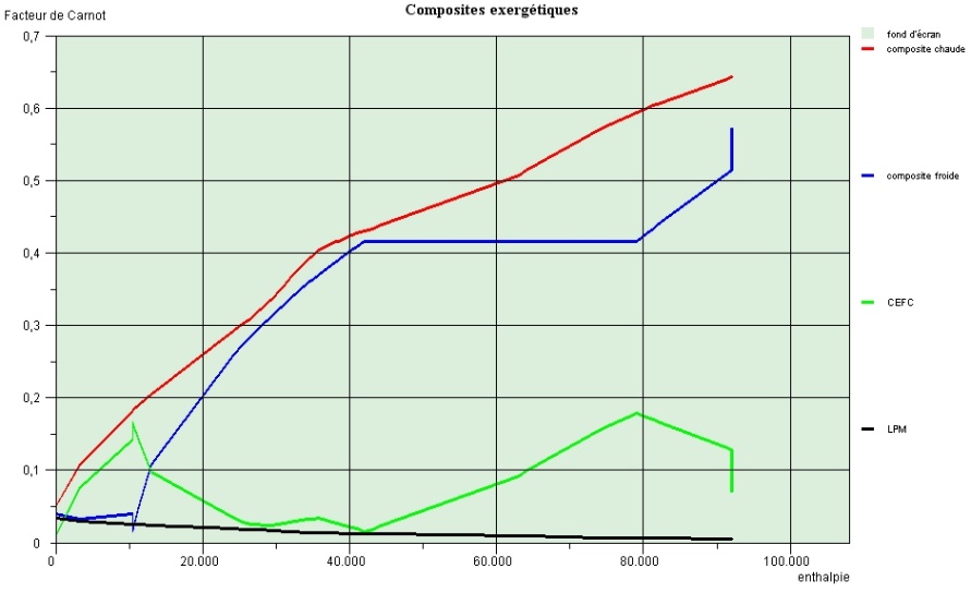
The hot and cold composite curves are constructed by adding the enthalpies available per temperature level, in the hot and cold streams, respectively. In the figure opposite, the hot composite curve is in red, above the cold composite curve in blue. Their relative positions are characteristic of the system, and the pinches appear at the places where the curves come the closest together (there are two in this example).
The curve showing the difference in Carnot factors, in green on the figure, can be constructed by subtracting the cold composite from the hot composite. The system irreversibilities are exactly equal to the area under this curve. You can also see a black curve, called the Minimum Pinch Points, which is used in the optimization method to distinguish two different types of irreversibilities. The first, called component irreversibilities, are characteristic of component operation, while the second, called system irreversibilities, are specific to the system architecture. Distinguishing between the two types of irreversibilities shows how much system-specific freedom you have to work around particular technological constraints, with no detriment in terms of energy.
As we said, the pinch points correspond to the most constrained zones of the system. Knowing where they are tells you immediately which streams play a critical role in the global configuration, and which system zones require special care during the design phase.
By displaying the pinch points in a way that is easy to visualize from a physics standpoint, this method provides a valuable guide replacing older heuristic methods that often required numerous iterations.
Based on the results obtained in the previous two steps, process modifications can be considered. Modifications are helpful if you can shift the pinch point(s) and reduce the utility stream, or increase the production of useful energy. Iterations are then performed between the time when the model parameters are reset in the simulator and steps 2 and 3 of the optimization method.
The fourth step consists of matching the streams to construct the heat exchangers. This relatively long and complex step should not be undertaken until the model parameters are deemed satisfactory. The process is facilitated by using the exchange blocks presented below.
In this note, we will not present the optimization method in great detail, partly because the theoretical bases use advanced notions of exergy and irreversibilities, and also because it is difficult to put together examples that are both easy to understand and sufficiently complex to require optimization. Given that these examples have to be simplified for instructional purposes, the value of the optimization method is not clearly apparent, especially if the solution can be arrived at simply by intuition and physics sense.
For more information, please see the documents listed in the references, in particular chapter 22 of the book " Energy Systems ", which presents the method and explains a step-by-step example of a heat recovery steam generator (HRSG) like those used to produce steam in combined cycles or in cogeneration plants. In an HRSG, the steam is produced at 2 to 4 pressure levels, which can be selected freely within certain limits. The steam properties are highly non-linear functions of temperature and pressure, the steam flow rates can vary depending on the operating conditions, and the heat exchanger matching possibilities are numerous. Moreover, whereas conventional boilers must satisfy exhaust temperature constraints, and therefore cannot be totally optimized from a thermal standpoint, HRSGs must satisfy pinch point constrains, so that when optimizing, you must take into account both the steam cycle and the heat exchange with the exhaust.
Using the method in Thermoptim
All of the functions specific to optimization are accessible from the optimization window (Special menu). They work in close coordination with the simulator, so you can easily modify the system parameters.
To get access to the optimization screen, type Ctrl M or select "Optimization tools" in the "Special" menu. The optimization screen is the following:
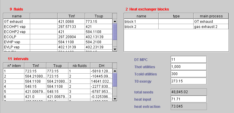
It is comprised of three main tables:
- the fluid table contains all the exchange fluids in which the "pinch method fluid" checkbox is selected. These are the fluids which are processed by the variant of the Problem Table Algorithm implemented in Thermoptim.
- the interval table contains the list of the intervals which are built by the PTA variant. It will be explained in more detail later
- the heat exchanger block table contains the exchange blocks which can be defined in order to facilitate fluid matching in heat exchangers.
In the lower right part of the screen appear several fields, five of which are editable:
- DT MPL is the minimum pinch value used for plotting the minimum pinch locus. By default it is set to 11 K
- Thot utilities is the temperature used to plot the hot utilities target (heat input requirements). By default it is set to 1000 K
- Tcold utilities is the temperature used to plot the cold utilities target (heat extraction requirements). By default it is set to 300 K
- T0 exergy is the value used for temperature reference in exergy calculations. By default it is set to 273.15 K (0 °C)
- total needs represents the sum of all the enthalpies of the cold fluids
- heat input is the value of the additional heat which may have to be provided to the hot fluids if the total needs exceed the heat available when the pinches are taken into account. This value is also often referred to as the "energy target".
- heat extraction represents the value of the heat which must be extracted from the system by cold utilities. It should be noted that the existence of pinch points explains that, as shown above, there may be at the same time a need for a heat input (at high temperature) and for a heat extraction (at low temperature).
Fluid table
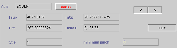
When you double-click on one of the fluids listed in the fluid table, the following frame appears:
It summarizes the data which is processed by the PTA and cannot be directly modified by the user, as it is built from the corresponding process which can be shown by clicking on the "display" button.
Intervals
Interval analysis plays an important role in pinch methods, as they allow one to understand how the different fluids are distributed. In particular the analysis of the intervals around the pinch points is of basic importance for efficiently matching fluids in heat exchangers. The intervals can be displayed either from the optimization frame, or from the charts themselves, by double-clicking on the diagram: the corresponding temperature is calculated, and the interval in which it is contained is displayed.
When you double-click on one of the lines of the interval table, the following screen appears:
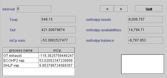
In the upper left zone are shown the number of the interval, its temperature limits Tsup and Tinf, and the algebraic sum of the thermal capacity flow rates mCp of the different fluids which are contained in the interval.
On the right are indicated the sum of the enthalpy needs and availabilities in the interval and the corresponding enthalpy balance.
The list of the fluids which are located close to the interval or cross it is displayed in the table with the value of their thermal capacity flow rate mCp. If you double-click on one of them, the corresponding process frame is shown.
Heat Exchanger Blocks
Heat exchanger blocks have been introduced in order to facilitate heat exchanger matching when a main process exchanges heat with several processes as for instance when one seeks to recover heat from gas turbine flue gases. In such a case the main hot fluid has to be divided (in series and/or in parallel) in several subprocesses to be matched with the different cold fluids. The role of the heat exchanger blocks is to provide assistance for dividing the main exchange process: one begins by grouping the fluids to be matched in blocks which are balanced at the enthalpy level; in a second step, the choice is made between series or parallel matching, and lastly the main fluid can be further divided.
Heat exchanger blocks are only used as part of the optimization method. They differ from the classical heat exchangers which are accessible from the main project screen. When the heat exchanger blocks have been defined, it is possible to divide the main process in as many subprocesses as required. Once this division is made, the classical heat exchangers can be easily built from the block frame.
The heat exchanger block frame looks as follows:
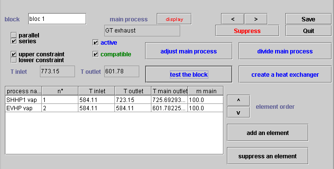
The name of the block appears in the upper left zone. On its right is the double-clickable field defining the main process (here "GT exhaust"), which may be displayed by clicking on the red button "display".
Below the block and main process names are located checkboxes which allow one to characterize the block: its elements may be matched in series or in parallel, and the block may be "upper" or "lower constraint" as explained below. The block may be "active" or not: only those blocks which are active are taken into account in the optimization method for the mixed problem when some heat exchangers are set. If the block is balanced at the enthalpy level and the temperatures of the different fluids comply with the pinch constraints, the block is "compatible".
On the lower left part of the frame is a table where are listed the different fluids which are to be matched with the main process. They can be added either by double-clicking in the table headband or by clicking on the button "add an element". They can be removed by clicking on the button "suppress an element". The fluid order may be modified by selecting one of them and shifting it using the two arrows on the right of the table. If you double-click in the table, the process corresponding to the fluid is shown.
Four blue buttons allow one to use the block:
- the button named "adjust main process" allows you to adjust the block enthalpy balance by modifying the inlet or outlet temperature of the main process. Thermoptim calculates the total enthalpy corresponding to the different elements which have been selected and sets that of the main vein to that value. If the "upper constraint" is selected, the minimum temperature of the vein is modified (the outlet one for a hot fluid, and the inlet one for a cold one). If the "lower constraint" is selected, this is done conversely.
- The button named "test the block" allows you to check the block consistency. Before activating it, it is necessary that the main process be adjusted by clicking on the previous button. Thermoptim checks the temperature compatibility between the main vein and the different block elements.
- Once a block is valid, it is possible to divide it into smaller blocks matching a part of the main vein and one of each block elements. If the "series" checkbox is selected, the main vein is divided in series into as many parts as there are block elements, of the same flow rate as the main vein, the intermediate temperatures being calculated. If the "parallel" checkbox is selected, the main vein is divided in parallel into as many branches as there are block elements, of the same temperatures as the main vein, their flow rate being calculated proportionally to the enthalpy of the divided block. Furthermore, you can ask Thermoptim to automatically build the divider and the mixer which connect the main vein divided branches.
Thermoptim automatically names the new types which it creates, adding _0, _1… to the existing names, except for the mixer (MIX_xxx) and the divider (DIV_xxx). If a type of that name already exists, it is modified.
- the fourth button named "create a heat exchanger" allows you to automatically start building the classical heat exchanger corresponding to a block comprised of a single element. If the two fluids of the block are already connected in an existing heat exchanger, a message warns you. In any case, the heat exchanger screen is shown. If it is created, you have to finish defining it by selecting the constraints and the type of calculation before calculating it. By default, the heat exchanger type is created of the counterflow type, but you can change it if you wish to do so.
Optimization Menus
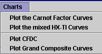
Currently the following menus are available:
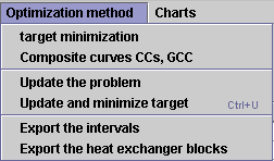
- target minimization corresponds to the shifted temperature PTA
- composite curves CCs, GCC builds up the composite curves
- update the problem updates the optimization elements from the process table
- update and minimize the target combines the third and first items
- Export the intervals creates a text file named "interv.txt" in subdirectory "pinch" containing all the information on the intervals
- Export the heat exchanger blocks creates a text file named " HXblock.txt" in subdirectory "pinch" containing all the information on the heat exchanger blocks, as well as preliminary computations of the exchanger characteristics (effectiveness, NTU, LMTD, UA value)
- plot the Carnot Factor curves plots the exergy composite curves
- plot the mixed HX-TI Curves plots the composite curves obtained when part of the heat exchanger network is set.
- plot CFDC plots only the Carnot Factor Difference Curve
- plot grand composite curves plots these curves
The two latter menu items are enabled only when either the Carnot Factor or the mixed HX-TI curves have been calculated.
References
GICQUEL R., Energy Systems: A New Approach to Engineering Thermodynamics, January 2012, CRC Press, ISBN-13: 978-0415685009.
GICQUEL R., Méthode d’optimisation systémique basée sur l’intégration thermique par extension de la méthode du pincement : application à la cogénération avec production de vapeur. Revue Générale de Thermique, tome 34, n° 405, octobre 1995.
GICQUEL R., MODICS. Généralisation de la méthode d’optimisation systémique aux systèmes
thermiques avec échangeurs imposés. Revue Générale de Thermique, tome 35, p. 423-433, 1996.
LEIDE B., GICQUEL R., Systemic approach applied to dual pression HRSG, International Gas Turbine & Aeroengine Congress and Exhibition, Orlando, Florida, 2-5 June 1997
LINNHOFF B., Use pinch analysis to knock down capital costs and emissions, Chemical Engineering Progress, august 1994, pp. 32 – 57
LINNHOFF B., HINDMARSH E., The pinch design method for heat exchanger networks, Chemical Engineering Sc., Vol. 38, n° 5, pp. 745-763, 1983.
LINNHOFF B., User Guide on Process Integration for the Efficient Use of Energy, Pergamon Press, Oxford, 1982.