Introduction

You have so far studied the simple cycle of the steam plant. You will now see how it can be improved, our aim being to minimize irreversibilities.

We have seen that the real engine cycles deviate significantly from the Carnot cycle, the differences coming from, among other things, the following points:

• in practice, there must be a certain temperature difference between the machine and the hot and cold sources
• it is exceptional that hot and cold sources can be considered as isothermal: most often it is a fluid which exchanges heat between two temperature levels
• when compression and expansion are adiabatic, they are not reversible due to mechanical irreversibilities

In practice, the modifications of the elementary cycles essentially concern:

• on the one hand on the reduction of temperature differences both with the outside of the system and internally
• and on the other hand on the splitting of the compressions and the detents

Reference cycle

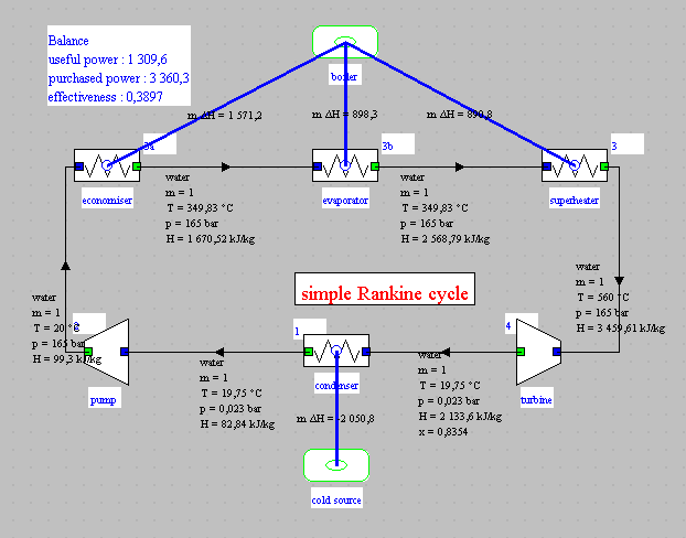
The reference cycle that we will use for steam power stations is a variant in terms of configuration of that presented in guided exploration S-M3-V7: the low pressure is set at 0.023 bar, the high at 165 bar, and the superheat temperature is 560 ° C, as shown in this diagram (project and diagram files: "steam_ref.prj" and "steam_ref.dia").

Let us calculate for this cycle the value of Carnot's efficiency, with $Tc=15+\mathrm{273,15}=\mathrm{283.15 K}$ and $Th=1000+\mathrm{273,15}=\mathrm{1273.15 K}$ : $\eta =\mathrm{78 \%}$.

The actual efficiency is therefore close to 50% of the maximum theoretical efficiency.

Cycle with reheat

As we have seen above, it is possible to improve such a cycle by splitting the compressions and expansions.

Steam power plants with reheat apply expansion splitting.

A first idea to improve the Hirn cycle is to approach the Carnot cycle by conducting reheats. In this case, we begin by partially expanding the fluid, then it passes again into the boiler, where it is heated, at the new pressure, at the maximum cycle temperature. This operation can optionally be repeated several times.

This results in efficiency gains of a few percent, and most importantly, as shown in the chart, increased quality at the end of expansion, which is always valuable to extend the life of turbine blades, for which liquid droplets are abrasive.

The price however is a higher complexity, but as the expansion must be staged anyway, this improvement has no major technological impact on the power plant.

Loading the model

Loading a cycle with reheat model.

Click on the following link: Open a file in Thermoptim

Cycle plot in the water (h, ln(P)) chart

First step: loading the water (h, ln(P)) chart

Click this button

Second step: loading the reference cycle and the cycle with reheat

Click this button

You get the plot of the cycles in the (h, ln (P)) chart: the new cycle in black and the refernce cycle in blue.

We can observe the clear increase in the quality at the end of the expansion mentioned above.

Cycle with reheat setting

The setting of the cycle with reheat is very close to that of the reference cycle, a variant of which was presented in the guided exploration S-M3-V7.

The main change concerns the modeling of the turbine. For the sake of simplicity, we have considered in the reference model that it has a constant isentropic efficiency whatever the high and low pressures, but this hypothesis can be improved.

Polytropic concept

To correctly model the reheat, we will use a new notion, that of polytropic efficiency.

For a turbine, the isentropic efficiency is defined as the ratio of the actual work provided by the turbine to the work it would have provided if the adiabatic expansion was perfect.

Knowing the isentropic efficiency ηs provides no indication of the law followed by the fluid during the irreversible expansion. To be able to do this, you have to make additional assumptions.

One of the most common leads to the widely used notion of polytropic, which may cover slightly different definitions depending on the authors.

The hypothesis that we give here is to consider that the irreversibilities are uniformly distributed throughout the expansion, which amounts to supposing that, during any infinitely small stage of the transformation, the isentropic efficiency keeps a constant value, by definition equal to the polytropic efficiency $\eta p$ which thus appears to be an infinitesimal isentropic efficiency.

For multi-stage machines with a large number of stages constructed in a similar manner, as in the case of a steam turbine, this efficiency has a clear physical meaning: it is, in a way, the elementary efficiency of a stage.

Knowing the polytropic efficiency of a stage, it is possible to determine the isentropic efficiency of a multi-stage machine, which varies according to the number of stages, itself linked to the expansion ratio.

Modeling a multi-stage turbine according to a polytropic approach is therefore more realistic than assuming that its isentropic efficiency is constant.

Transition from the polytropic approach to the isentropic approach

In Thermoptim, you can set compression or expansion by choosing one approach or another, and switch from one to the other without difficulty as you will see.

In view of what has just been said, the two high and low pressure turbines are modeled according to the polytropic reference in the reheating cycle model, their polytropic efficiency being equal to 0.805.

Open the high pressure turbine screen to see how Thermoptim calculates the equivalent isentropic efficiency.

For the continuation of this guided exploration, then return to the initial configuration: polytropic reference, polytropic efficiency equal to 0.805, and calculation mode "Set the efficiency and calculate the process".

Cycle with reheat balance

With this setting and an intermediate pressure of 10 bar, the result of the reheating cycle modeling is provided by Thermoptim: the efficiency goes from 38% for the reference cycle to 41.8%.

First law balance

Increase in useful power

Reheat has the effect of increasing the useful power.

For comparison, this synoptic view provides you with the performance values ​​of the reference unit.

Parametric study of the cycle with reheat

Exercise: look for the intermediate pressure that leads to optimal performance.

Check whether the intermediate pressure of 10 bar has been chosen correctly, by studying its influence on cycle performance (efficiency and power).

Conclusion

This exploration allowed you to see the interest of the splitting of the expansion followed by a reheat on the performance of the plant.

It also showed you that it is better to model multi-stage turbomachines using a polytropic approach.