Introduction
Organic Rankine cycles are variants of the water vapor cycles, which are used when the hot source from which one wishes to produce mechanical power is at low or medium temperature, or when the installed power is low and steam installations are no longer economical.
When the temperature of the hot source drops, or that the installed power decreases, typically below ten MW, the performance of steam vapor cycles deteriorates, and it becomes preferable to use other thermodynamic fluids.
Since many of these are organic in nature, it is customary to qualify these organic cycles, but other types of fluids, such as ammonia or carbon dioxide, can be used.
Here we present an example of an ORC cycle intended to generate electricity from the thermal gradient of the oceans.
OTEC stands for Ocean Thermal Energy Conversion; its equivalent in French is Energie Thermique des Mers (ETM)
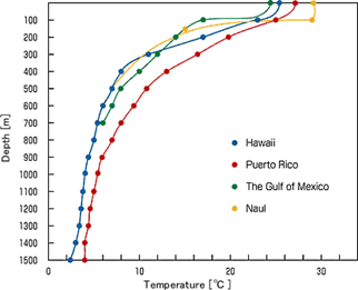 OTEC cycles are
designed to generate electricity in warm tropical waters using the
temperature difference between water at the surface (26-28 °C) and in
depth (4-6 ° C), from 1000 m as shown by this figure.
OTEC cycles are
designed to generate electricity in warm tropical waters using the
temperature difference between water at the surface (26-28 °C) and in
depth (4-6 ° C), from 1000 m as shown by this figure.
Closed cycles use hot water at about 27 °C to evaporate a liquid that boils at a very low temperature, such as ammonia or an organic fluid. The vapor produced drives a turbine, then is condensed by heat exchange with cold water at about 4 °C from deeper layers of the ocean.
In all cases, the need to convey very high water flow rates and pump cold water at great depth induces significant auxiliary consumption. Optimization of an OTEC cycle is imperative to take into account those values.
The thermodynamic cycle is similar to the one we have studied for steam plants except that the working fluid is ammonia. The sizing of heat exchangers is of course even more critical given the very small temperature difference between hot and cold sources. Pinch values should be as low as possible while remaining realistic.
Closed OTEC cycle diagram
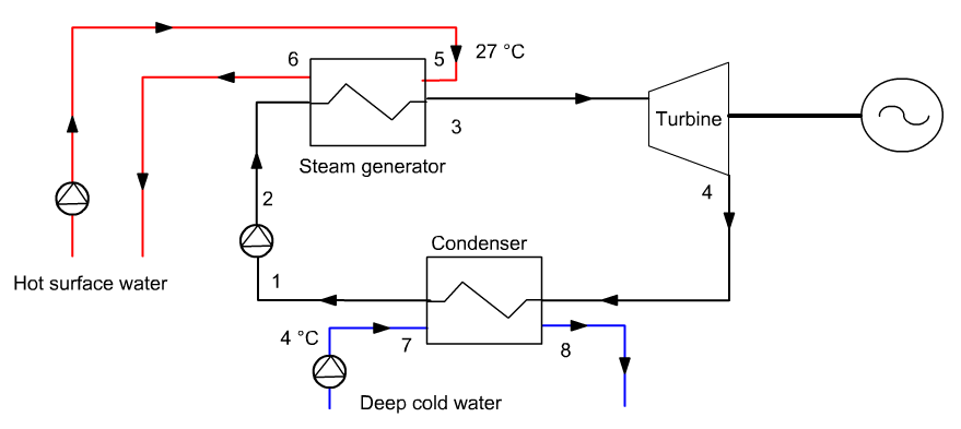 At point 1 at the condenser
outlet, the working fluid is in the liquid state.
At point 1 at the condenser
outlet, the working fluid is in the liquid state.
The pump compresses the ammonia to 9 bar.
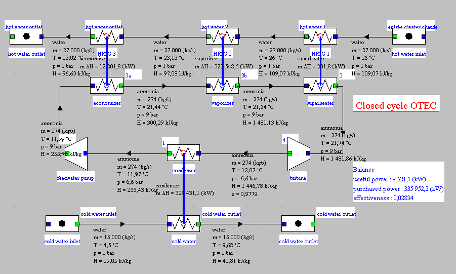
The steam generator is a triple exchanger ensuring heating in the liquid state, vaporization and a slight superheating of the ammonia.
The pump and the turbine can be assumed to be adiabatic. As for the steam generator and the condenser, we can at first guess that they are isobaric.
Loading a model
Load the model
Click on the following link: Open a file in Thermoptim
You can also:
- either open the "Project files/Example catalog" (CtrlE) and select model m8.5 in Chapter 8 model list.
- or directly open the diagram file (OTEC_CC_ammonia.dia) using the "File/Open" menu in the diagram editor menu, and the project file (OTEC_CC_ammonia.prj) using the "Project files/Load a project" menu in the simulator.
Model settings
In this section, we will mainly focus on the configuration of heat exchangers.
ORC cycle settings
At point 1 at the condenser outlet, the working fluid is in the liquid state, at a pressure of 6.6 bar. At this pressure, the saturation temperature of the ammonia is approximately 12 ° C. To make sure that the point is in the liquid state, we set it to the imposed saturation temperature, with an approach of -0.1 ° C from the saturation.
The high pressure is 9 bar. The pump is assumed to be perfect and the isentropic efficiency η of the turbine is equal to 0.9.
The setting of the ORC cycle does not pose any particular problem.
Setting the condenser
Now let's take a look at the configuration of the condenser which is a relatively simple exchanger.
Steam generator settings
The pressurized ammonia is brought to high temperature in the steam generator, the heating comprising the following three stages:
- liquid heating from almost 12 ° C to 21.54 ° C, boiling point at 9 bar: evolution (2–3a) ;
- vaporization at constant temperature 21.54 ° C: evolution (3a–3b) ;
- slight superheating from 21.54 °C to 21.74 °C.
Let us examine how this triple exchanger is set.
We know the state of the ammonia entering and leaving each part of the exchanger, as well as its flow rate, which are therefore set values.
Point 3b is set analogously, with the proviso that the quality is equal to 1, to indicate the state of vapor.
The flow rate and the inlet temperature of the hot water into the superheater are known, and therefore set, which makes it possible to determine the temperature of the water from the outlet point of this exchanger ("hot water 1"), which is also the inlet point of water in the next exchanger, the evaporator.
Since five quantities are known in this exchanger, it can also be calculated, which makes it possible to find the temperature of the water at the outlet point of this exchanger ("hot water 2"), which is also the inlet point of water in the next exchanger, the economizer.
Step by step, the steam generator can thus be calculated.
Pinches in exchangers
The minimum temperature difference between the hot fluid and the cold fluid is called an exchanger pinch. As a general rule, pinch values of the order of at least 5 to 10 °C are retained, but for an OTEC cycle, the temperature difference between the two hot and cold sources is so small that one is led to choose much lower values.
Open the "condenser" exchanger and determine the pinch value by calculating the minimum temperature difference between the hot fluid and the cold fluid.
What is the pinch value in the condenser?
In the triple exchanger that constitutes the steam generator, check that the pinch is at the level of the evaporator.
Open the "evaporator" exchanger and determine the pinch value by calculating the minimum temperature difference between the hot fluid and the cold fluid.
What is the pinch value in the steam generator?
As you can see, these two values are very small. To reach them, the surfaces of the heat exchangers must be very large.
Cycle plot in the (h, ln(P)) chart
First step: loading the diagram of the ammonia (h, ln(P)) chart
Click this button
You can also open the diagram using the "Interactive Charts" line in the "Special" menu of the simulator screen, which opens an interface that links the simulator and the diagram. Double-click in the field at the top left of this interface to choose the type of diagram desired (here "Vapors").
Once the diagram is open, choose "ammonia" from the Substance menu, and select "(h, p)" from the "Chart" menu.
Second step: loading a pre-recorded cycle corresponding to the loaded project
Click this button
You can also open this cycle in the following way: in the diagram window, choose "Load a cycle" from the Cycle menu, and select "cycleOTEC_NH3.txt" in the list of available cycles.
We find the usual look of the cycle. Since the superheating is very low, the expansion takes place almost entirely in the liquid-vapor equilibrium zone.
Fluid change
In the previous model, the fluid was ammonia. We will now see how it is possible to change the fluid without having to completely reconstruct the model.
However, as the saturation pressure law of the new fluid will be different from that of ammonia, a certain number of elements will have to be set differently.
Model settings
Let's start by replacing the ammonia with butane.
To change the fluid, go to the diagram editor and delete the links which connect the components of the ammonia circuit.
Select one of the components, for example the turbine, and display its properties (F4 key or menu Edit/Show properties).
Click on the "outlet port" tab, then in the "substance name" field, either enter butane instead of ammonia, or double-click and select "butane" from the list of condensable vapors.
Then click on "Apply".
Place the mouse on the small green rectangle located to the left of the turbine component and click. It turns into target. Keeping the click, drag the link that appears to the small blue rectangle that corresponds to the inlet point of the condenser
By doing this, you propagate the new substance from the turbine component to the condenser component, which you can check by displaying the properties of the condenser (F4 key or menu Edit/Show properties).
Repeat the operation by connecting the condenser to the pump ("feedwater pump" component), then this to the economizer, and so on until the turbine is reconnected upstream.
Open the Diagram / simulator interface via the Special menu of the diagram editor, and click on the "Update the element table" button, then click on the "Update the simulator from the diagram" button.
Thermoptim begins to carry out the updates, then asks you, for each of the points concerned, to confirm the change of substance.
Confirm. Once the update is done, the substance change is done in both the diagram editor and the simulator
If you display the values in the diagram editor, you see that the vaporization and condensation temperatures are 74.7 °C and 61.3 °C, that is to say much too high.
We will now determine the high and low pressures of the butane cycle.
Open point 4 at the turbine outlet and enter 12 °C in the temperature field, then click on "set the saturation pressure".
The value of the saturation pressure is then calculated: 1.594 bar.
Then click on "unconstrained", and enter 1.6 bar as the pressure value, then calculate the point.
Open point 2 at the pump outlet and enter 22 ° C in the temperature field, then click on "set thesaturation pressure".
The value of the saturation pressure is then calculated: 2.218 bar.
Then click on "unconstrained", and enter 2.2 bar as the pressure value, then calculate the point.
Then recalculate several times in the simulator screen until the balance stabilizes. Answer "OK" to the error messages that are displayed until the model is completely reset.
Note that we have only used "set the saturation pressure" as a provisional setting and not definitive, because, in cycle models, it is generally better to consider pressures as known rather than temperatures. This comes in particular from the fact that the isobar is the reference evolution for heat transfers or open system combustions.
Butane flow adjustment
The model we have just obtained is consistent with the one whose working fluid was ammonia, but its power is much lower: 3.13 MW instead of 9.6 MW.
It is therefore necessary to approximately triple the butane flow rate, which you can do by modifying it in the process whose flow rate is set, that is to say the economizer.
By entering a value of 840 kg/s, you get comparable power.
If you have a problem, load the new ORC cycle model with butane.
Loading the ORC cycle model with butane
CClick on the following link: Open a file in Thermoptim
You can also:
- either open the "Project files/Example catalog" (CtrlE) and select model m8.6 in Chapter 8 model list.
- or directly open the diagram file (OTEC_CC_butane.dia) using the "File/Open" menu in the diagram editor menu, and the project file (OTEC_CC_butane.prj) using the "Project files/Load a project" menu of the simulator.
You can now compare this cycle with the ammonia cycle.
Cycle display in butane chart
To display the cycle in the butane chart, you can do the following.
Start by closing the ammonia (h, ln (P)) chart window.
Open the interface between the simulator and the diagrams by activating the "Interactive charts" line in the "Special" menu of the simulator.
Double-click in the field at the top left of this interface to choose the type of diagram desired (here "Vapors").
Once the chart is open, choose "butane" from the substance menu, and select "(h, p)" from the "Chart" menu.
Return to the interface between the simulator and the charts and click on "Update the point table".
Deselect all the points whose substance is water, then click on "Update the chart from the simulator". The points then appear in the chart.
Connect them together by selecting the "Connected points" line in the "Cycle" menu. The points are interconnected, but the cycle is not completely closed.
You can also click on this button
You can also open this cycle as follows: in the diagram window, choose "Load a cycle" from the Cycle menu, and select "cycleOTEC_but.txt" from the list of available cycles. Then click on the "Connected points" line in the Cycle menu.
As you can see, the expansion takes place entirely in the vapor zone, whereas it took place in a humid zone with ammonia. This comes from the shape of the reversible or isentropic adiabatic curves.
Conclusion
This exploration allowed you to discover an ORC cycle modeled in Thermoptim and to see how it is possible to change the working fluid.
VYou can use this model to analyze the sensitivity of the model to various parameters, such as the isentropic efficiency of the turbine.
Open the "condenser" exchanger and examine its setting.
We know the state of the ammonia entering and leaving the condenser, as well as its flow rate, which are therefore set values.
We will also assume that the cooling water flow is 15 t/s (15,000 kg/s). This is water pumped to a depth of about 1000 m, at a temperature of 4 °C. These two quantities are therefore also set, and five constraints are thus set.
The only value to calculate is the water outlet temperature.