Introduction
The objective of this exploration is to guide you in your first steps of using Thermoptim, by making you discover the main screens and functionalities associated with a model of simple steam power plant.
You will discover how the screens of points and processes can be set and calculated, the concepts of useful and purchased energies making it possible to draw up global energy balances.
You will visualize the cycles in the thermodynamic (h, ln (P)) chart and you will carry out studies of sensitivity of the cycle depending on the outside temperature and the high pressure.
A steam plant operates on the Hirn (or Rankine with superheating) cycle, which uses a condensable fluid, water, which is cooled at a pressure and temperature sufficient for it to be fully liquefied before compression.
In such conditions, the compression work becomes almost negligible compared to the expansion work (whereas it represents around 60% in a gas turbine). The compressed liquid is vaporized and superheated in the boiler by heat exchange with the hot source, then expanded and condensed.
Technological aspects
 At point 1
at the condenser outlet, the water is in the liquid state, at a
temperature of about 27 ° C. At this temperature, the water saturation
pressure is very low (0.0356 bar).
At point 1
at the condenser outlet, the water is in the liquid state, at a
temperature of about 27 ° C. At this temperature, the water saturation
pressure is very low (0.0356 bar).
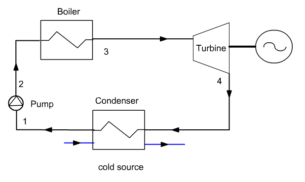
This diagram shows that such a plant comprises four components: a pump, a boiler, a turbine and a condenser, crossed by the same flow of water.
The pump and the turbine can be assumed to be adiabatic. As for the boiler and the condenser, we can at first guess that they are isobaric.
The pump is generally of the centrifugal, multi-stage type, given the very high compression ratio to be achieved.
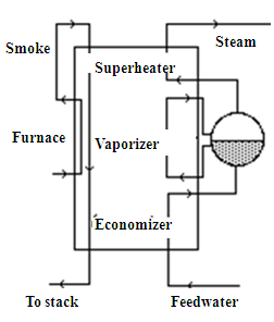
The boiler, generally of the water tube type, performs three successive functions:
- heating the pressurized feedwater to the vaporization temperature at the corresponding pressure;
- vaporize the water;
- and finally superheat it to the desired temperature.
It therefore behaves like a triple exchanger, and can be represented from the point of view of heat exchanges by the diagram in the figure.
Loading the model
The model is loaded by opening the diagram file and an appropriately configured project file.
Start by loading the model, then perform the other proposed activities.
Loading the model
Click on the following link: Open a file in Thermoptim
You can also:
- either open the "Project files/Example catalog" (CtrlE) and select model m3.2 in Chapter 3 model list.
- or directly open the diagram file (steam_light.dia) using the "File / Open" menu from the diagram editor menu, and the project file (steam_light.prj) using the "Project file/Load a project "from the simulator menu.
Discovery of Thermoptim
The diagram editor allows you to describe graphically and qualitatively the system studied. It includes a palette presenting the different representable components and a work panel where these components are placed and interconnected by vector links.
The simulator allows you to quantify and then calculate the model described in the diagram editor. It includes the lists of the different points, processes, nodes and exchangers of the model.
Display these two windows and study their content.
Refer for more explanations to the Thermoptim discovery exploration accessible from the menu at the top left of the browser screen.
Main components of the model
How many main components does the cycle use?
Mechanical energy
What component (s) put mechanical energy into play?
Energies put into play
Enter the values in the text fields below. Your answer is evaluated against the correct value, with an interval corresponding to a precision which depends on the question.
Remember that the energies or powers received by a system are counted positively, and those it supplies to the outside are counted negatively. In Thermoptim screens, they are therefore positive or negative, depending on the case.
However, in these exercises, enter only the absolute values of the capacities involved (in kW)
What is the value of the power produced by the turbine?
What is the value of the power consumed by the pump?
Value of net mechanical power?
Value of the thermal power supplied to the evaporator?
Value of the total thermal power supplied?
Value of the efficiency?
Model settings
In this section, we will make the link between the model statement and the setting of the main points and processes
Settings retained
At point 1 at the condenser outlet, the water is in the liquid state, at a temperature of about 27 ° C. At this temperature, the water saturation pressure is very low (0.0356 bar).
Open point 1 and examine its setting.
Its pressure is equal to 0.0356 bar, and the option "set saturation temperature" has been chosen, the quality being equal to 0, to indicate the liquid state.
Recall that, for a pure substance in liquid-vapor equilibrium, the quality is defined as the mass of vapor divided by the total mass of liquid and vapor.
If you change the pressure value, and you recalculate the point, its temperature is automatically modified.
If you enter another value for the quality, between 0 and 1, for example 0.5, and recalculate the point, the temperature does not change, but the enthalpy h increases sharply.
The pump compresses liquid water to around 128 bar, which represents a considerable compression ratio (around 3600).
Open the "pump" process, and examine its setting.
It connects point 1 and point 2, and its setting is "adiabatic", "isentropic reference", with an isentropic efficiency equal to 1.
It is in point 2 that the pressure of 128 bar is defined.
Open point 2. . Its setting is "unconstrained", which means that the pressure and its temperature are independent.
When the "pump" process is calculated, the temperature of point 2 is determined.
If you change the pressure of point 2, for example by entering 160 bar, the new end of compression temperature is calculated. It differs very little from the previous one.
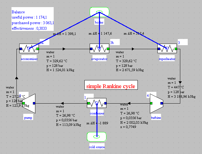
The pressurized water is then brought to high temperature in the boiler, the heating comprising the following three stages:
- heating of the liquid from around 27 °C to around 330 °C, boiling point at 128 bar: evolution (2–3a) ;
- vaporization at constant temperature 330 °C: evolution (3a–3b) ;
- superheating from 330 °C to 447 °C.
Point 3a is configured in a completely analogous way to point 1, the option "set the saturation temperature" being chosen, and the quality being equal to 0, to indicate the liquid state.
Point 3b is set analogously, with the proviso that the quality is equal to 1, to indicate the state of vapor.
The setting of point 3 is completely defined in this statement: its pressure and temperature are known so that you just enter them and calculate the point.
The evolution (3–4) is an irreversible adiabatic expansion from 128 bar to 0.0356 bar, with isentropic efficiency η = 0.9.
This evolution is modeled by the "turbine" process.
The upstream state of the fluid is that of point 3, the pressure and temperature of which are known.
For the downstream, point only the pressure is known.
Open the "turbine" process, and examine its setting.
It connects point 3 and point 4, and its setting is "adiabatic", "isentropic reference", with an isentropic efficiency equal to 0.9.
It is in point 4 that the outlet pressure of 0.0356 bar is defined.
The outlet state is two-phase, which means that the temperature is equal to that of saturation at this pressure. The quality, equal to 0.775, is determined when calculating the process.
If you change the value of the isentropic efficiency, the new exit quality is calculated.
Cycle plot in the (h, ln (P)) chart
First step: loading the water (h, ln (P)) chart
Click this button
You can also open the diagram using the "Interactive Diagrams" line in the "Special" menu of the simulator screen, which opens an interface that links the simulator and the diagram. Double-click in the field at the top left of this interface to choose the type of diagram desired (here "Vapors").
Once the diagram is open, choose "water" from the substance menu, and select "(h, p)" from the "Graph" menu.
Second step: loading a pre-recorded cycle corresponding to the loaded project, the layout of which has been previously refined in order to be more precise
Click this button
You can also open this cycle as follows: in the diagram window, choose "Load a cycle" from the Cycle menu, and select "cycle_lightEnThin.txt" from the list of available cycles. Then click on the "Connected points" line in the Cycle menu.
cycle identification on the diagram
Identification of some characteristic points in the chart
Enter a point in liquid zone
What is the point in two-phase zone?
What is the point with the highest temperature?
Cycle analysis
Compression in the liquid state is represented here by the very visible almost vertical segment (1–2).
If one neglects the pressure drops in the steam generator or the boiler, the overall heating corresponds to the horizontal (2–3). The three parts representing the economizer, the evaporator and the superheater appear very distinctly.
The irreversible expansion results in a steeper curve than the reversible adiabatic, point 4 being located in the liquid-vapor equilibrium zone.
Finally, isobaric condensation is also horizontal.
Here you find the values that you had estimated during the previous exercise of building the cycle on a diagram.
Influence of the condensing temperature
The previous model assumed that the outside temperature was low enough to condense around 20 ° C, which corresponds to a winter situation. We are now interested in the operation of the plant in summer, the condensing temperature rising to 40 ° C (and the condensing pressure to 0.074 bar). The corresponding project is loaded by emulating Thermoptim.
Set the model by yourself, knowing that, if you encounter a difficulty, the corrected project can be loaded by emulating Thermoptim.
Once the settings have been made, in order for the modifications to appear in the diagram editor, hide the values, then re-display them, by selecting the menu line "Special/Show values" twice, or by typing twice the F3 key.
Loading the model
Click on the following link: Open a file in Thermoptim
You can also open the diagram file (steam_light40.dia) using the "File / Open" menu in the diagram editor menu, and the project file (steam_light40.prj) using the "Project files/Load a project" menu in the simulator.
Cycle display with condensation at 40 °C
Loading the cycle plot with condensation at 40 °C makes it possible to superimpose it on the initial cycle. In the (h, ln (P)) chart, the increase in the condensing pressure and temperature is clearly visible.
Click this button
You can also open this cycle as follows: in the diagram window, choose "Load a cycle" from the Cycle menu, and select "cycle_light40EnThin.txt" from the list of available cycles. Then click on the "Connected points" line in the Cycle menu.
Reduction in useful work
Increasing the condensing temperature has the effect of reducing useful work.
For comparison, this synoptic view provides you with the performance values of the plant condensing at 20 °C (first part of the exploration).
By what value does useful work decrease?
By what value does purchased power decrease?
First law balance
What is the value of the useful power?
What is the value of the purchased power?
What is the value of the efficiency?
Second step: clearing the condensing cycle at 40 ° C
For the rest of the scenario, we erase the condensing cycle at 40 °C
Click this button
You can also delete the unnecessary cycle by following these steps: Display the Cycle manager from the Cycle menu. Click on the "Update cycle table" button, and deselect the rows that you do not want to appear on the chart.
Influence of high pressure
The previous model assumed that the HP pressure was 128 bar.
We are now interested in the operation of the plant with an HP pressure of 150 bar, the condensing temperature being that of the initial model, that is to say 20 ° C (and the condensing pressure 0.0356 bar).
You will set the model by yourself, knowing that the corrected project can be loaded by emulating Thermoptim if you encounter a difficulty.
Loading the model
Click on the following link: Open a file in Thermoptim
You can also open the diagram file (steam_light150.dia) using the "File / Open" menu from the diagram editor menu, and the project file (steam_light150.prj) using the "Project files/Load a project" menu of the simulator.
Overlay of the new cycle in (h, ln (P)) chart
Loading the cycle plot with 150 bar high pressure makes it possible to superimpose it on the initial cycle.
In the (h, ln (P)) chart, the increase in the condensing pressure and temperature is clearly visible.
Click this button
You can also open this cycle as follows: in the diagram window, choose "Load a cycle" from the Cycle menu, and select "cycle_light150EnThin.txt" from the list of available cycles. Then click on the "Connected points" line in the Cycle menu.
Reduction in useful work
Increasing the pressure slightly decreases the useful work, but the purchased power drops more and the efficiency increases a little.
For comparison, this synoptic view provides you with the performance values of the plant condensing at 20 ° C (first part of the exploration).
By what value does useful work decrease?
By what value does purchased power decrease?
First law balance
What is the value of the useful power?
What is the value of the purchased power?
What is the value of the efficiency?
Determination of isentropic efficiency when the state of the outlet point is known
The initial model (HP = 128 bar, LP = 0.0356 bar) assumed that the isentropic efficiency of the turbine was known.
We are now interested in setting the model when we know not its value but that of the state of the outlet point (0.0356 bar, set saturation temperature, x = 0.83).
Enter these values in the screen for point 4, then recalculate it.
In the screen of the "turbine" process, select the option "Calculate the efficiency, the outlet point being known" at the bottom right, then recalculate the process.
what is the new value of the isentropic expansion efficiency? (enter its value between 0 and 1)
It is thus possible to configure an expansion process knowing either its isentropic efficiency, or the state of its outlet point.
Conclusion
This exploration allowed you to discover Thermoptim and to start using this software package to make settings for a simple model.
You can perform others to analyze the sensitivity of the model to various parameters, such as the isentropic efficiency of the turbine.
We recommend that you read the Thermoptim documentation, and in particular the first two volumes of its reference manual.
Other guided explorations will allow you to study variants of this cycle to improve performance.
Open the diagram editor and count the components of the model, excluding external sources.
This question has several answers, depending on whether we consider multizone exchangers as composed of one or more components