Introduction

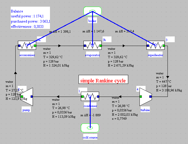
The purpose of this guided exploration is to guide you through your first steps in setting up a steam plant condenser.

It follows on from the guided exploration S-M3-V7 which presented the cycle of a single pressure steam plant, superheated at 447 ° C, whose synoptic view is given opposite.

Reminders on how to set the steam cycle

The setting is that of the S-M3-V7 guided exploration, the only difference being the representation of the exchanger corresponding to the condenser. Let us recall the main elements.

At point 1 at the condenser outlet, water is in the liquid state, at a temperature of approximately 27 ° C. At this temperature, the saturation pressure of the water is very low (0.0356 bar).

The pump compresses liquid water to around 128 bar, which represents a considerable compression ratio (around 3600).

The pressurized water is then brought to high temperature in the boiler, the heating comprising the following three stages:

heating of the liquid from nearly 27 ° C to about 330 ° C, saturation temperature at 128 bar: evolution (2–3a);
vaporization at constant temperature 330 ° C: evolution (3a – 3b);
superheat from 330 ° C to 447 ° C.

The following process (3–4) is an irreversible adiabatic expansion from 128 bar to 0.0356 bar, in a steam turbine with isentropic efficiency η = 0.9.

The liquid-vapor mixture leaving the turbine is finally condensed in a condenser, the modeling of which is the subject of this guided exploration.

Reminders on the calculation of exchangers using the NTU method

The method of calculating the exchangers that we recommend is called the Number of Transfer Units or NTU method.

It is presented in this page of the Thermoptim-UNIT portal, to which we suggest you refer if you do not remember it well.

Loading the model

Loading the model is done by opening the diagram file and a properly configured project file.

Load the model

Click on the following link: Open a file in Thermoptim

You can also:

either open the "Project files/Example catalog" (CtrlE) and select model m4.3 in Chapter 4 model list.
or directly open the diagram file (steam_cond.dia) using the “File/Open” menu in the diagram editor menu, and the project file (steam_cond.prj) using the “Project files/Load a project ”from the simulator menu.

Show diagram editor

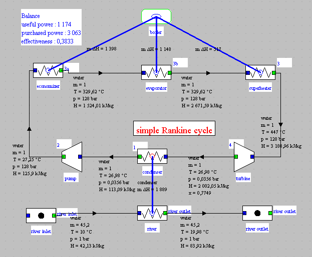
The model appears in the diagram editor.

We find the components of the steam cycle, plus, at the bottom, the condenser.

Two processes-points represent the inlet and outlet of the river water, the "river" exchange process corresponding to the heating of the river water passing through the condenser.

Reminders on the setting of exchangers

An exchanger performs the thermal coupling between two fluids, one which cools, the other which heats up. In the diagram editor, this coupling appears in the form of the blue link between the "condenser" and "river" exchange processes. Double-clicking on this link opens the exchanger screen.

The heat exchanger calculation screen has in its central zone two parts, the one on the left for the hot fluid, and the one on the right for the cold fluid.

Besides values of temperatures, flow rates, specific heats and enthalpies involved, there appear constraints on temperatures and flow rates that serve to guide heat exchanger calculations by allowing one to distinguish from among the problem variables those that are set and those that have to be calculated.

The following are possible types of heat exchangers: counter-flow, parallel-flow, crossed flows, mixed or unmixed Cpmin or Cpmax, and (p-n).

By default, we will assume that it is a counter-flow heat exchanger, even if in reality we are closer to cross flows. This choice only plays a second order on the results that interest us here.

In the lower left corner, appear:

three checkboxes allowing one to specify the absence or presence of implicit constraints on temperatures (see below).
A field for entering and/or displaying the value of the effectiveness

In the lower right corner, appear:

two checkboxes for setting the heat exchanger calculation mode: either "design" or "off-design".
We will only be interested here in "design" mode.

A heat exchanger connects two « exchange » processes. One of them is a hot fluid which corresponds to a substance that gets colder, while the other is a cold fluid that gets hotter. Once the coupling of the processes is made, the design problem is the following: it is necessary on one hand to conserve enthalpy in the heat exchanger, and on the other hand to respect some temperatures constraints.

Given that there are four temperatures (two for each fluid) and two flow rates, the problem has five degrees of freedom once the enthalpy is conserved. One can furthermore show that at least one of the two flow rates has to be set, otherwise the problem is indeterminable.

For temperatures, one can either set explicit constraints (for example temperatures of the inlet fluids), or implicit constraints (the value of the heat exchanger effectiveness, or the pinch minimal value).

To set a value to the effectiveness, enter the value in the epsilon field, and click on the button «set effectiveness». To set a «minimal pinch», all you have to do is select this calculation mode and enter the value of the desired minimum pinch in the field to the right of the "minimum pinch" option.

For the problem to have a solution, it is necessary to set a total of five constraints, among which there is a flow rate. If one of them is implicit (effectiveness or minimal pinch), four have to be explicit (3 temperatures and 1 flow rate, or 2 temperatures and 2 flow rates), or otherwise all five have to be explicit (a single flow rate or a single temperature is free).

These conditions are necessary, but non sufficient. This is why Thermoptim analyzes all the constraints proposed. If there is a solution, it will be found. Otherwise, a message tells the user that the calculation is impossible.

One can note that the design of heat exchangers is always made with the implicit hypothesis that thermophysical properties of the fluids remain constant in the heat exchanger, but this hypothesis is not made during the calculation of the processes. Therefore, when one recalculates a temperature on the basis on heat exchanger equations, slight differences may exist between the values displayed on the heat exchanger screen and that of the corresponding processes, or between the values of the enthalpies involved in both hot and cold fluids. If a high accuracy is required, one may have to make first a heat exchanger design calculation, and then iterate. Convergence is obtained fast.

Setting of the "condenser" exchanger

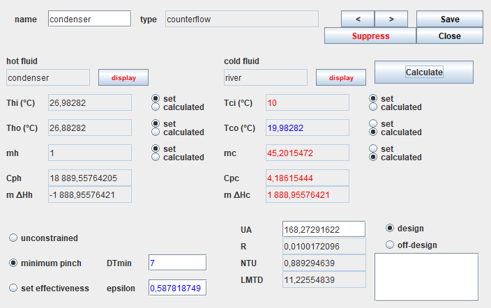
For the record, here is the condenser screen.

Let us take a look at its settings.

All the values concerning the hot fluid are known: its inlet and outlet temperatures and its flow rate, which sets three constraints.

We considered that the temperature of the river upstream of the condenser is known, which fixes a fourth. There is therefore only one degree of freedom.

In this first example, we have set a minimum pinch of 7 ° C, and we seek to determine the cooling water flow rate as well as the temperature of the water being discharged into the river.

The efficiency is epsilon = 0.589, the number of transfer units is NTU = 0.89, the heat capacity ratio is R = 0.01, and the product of the exchange surface area by the exchange coefficient is UA = 168.8 kW / K. The water flow of the river is equal to 45.2 kg / s. The LMTD logarithmic mean temperature difference is 11.2 ° C. The discharge temperature of the water is a little less than 20 ° C.

Other possible settings

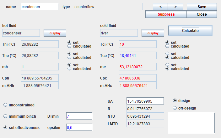
If we no longer set the minimum pinch, but for example an effectiveness equal to 0.5, the result is the following:

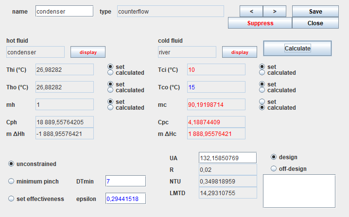
Coolant flow rate and LMTD increased a bit, while UA and NTU decreased slightly.

It is also possible to set no longer the minimum pinch or effectiveness , but the cooling water discharge temperature equal for example to 15 ° C.

To do this, this value must be modified in the "river 2" point screen and recalculated, then the exchanger must be set as unconstrained, the temperature Tco being set and no longer calculated. The result obtained is as follows:

The coolant flow rate almost doubled from the first case, and LMTD increased further, while UA and NTU decreased.

The coolant flow rate almost doubled from the first case, and LMTD increased further, while UA and NTU decreased.

In all the previous settings, we had the cooling water flow calculated. Now suppose we set it to 70 kg / s

To do this, you must modify this value in the screen of the "river 1" process-point and recalculate it, then configure the exchanger as unconstrained, the flow mf being imposed and no longer calculated. It is of course necessary that the temperature Tfs be calculated and no longer imposed. The result obtained is as follows:

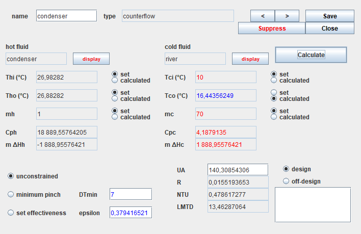
As you can see, the exchanger can be calculated in various ways depending on the parameters you want to set. What matters is to make sure that five constraints are set.

Design of a steam plant condenser