Introduction
The objective of this exploration is to guide you in your first steps of using Thermoptim, by making you discover the main screens and functionalities associated with a simple gas turbine model.
You will discover the layout of the screens of the points and the processes, the way in which they can be reconfigured and calculated, the concepts of useful and paying energies making it possible to draw up the global energy balances.
You will visualize the cycles in the thermodynamic diagram (h, ln (P)) and you will carry out studies of sensitivity of the cycle to the outside temperature, the turbine inlet temperature and the compression ratio.
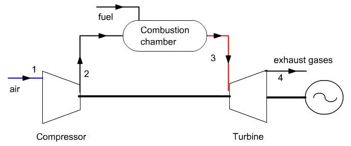 In
its simplest and most widespread form, a gas turbine (also called
combustion turbine) is composed of three elements:
In
its simplest and most widespread form, a gas turbine (also called
combustion turbine) is composed of three elements:
- a compressor, centrifugal or axial, which has the role of compressing ambient air to a pressure today between 10 and 30 bar;
- a combustion chamber, into which a gaseous or liquid fuel is injected under pressure, then burned with compressed air, with a large excess of air in order to limit the temperature of the exhaust gases;
- a generally axial turbine in which the gases leaving the combustion chamber are expanded.
In this form, the gas turbine constitutes an internal combustion engine with continuous flow. It will be noted that the compression work represents approximately 60% of the expansion work.
The name gas turbine comes from the state of the working fluid, which always remains gaseous, and not from the fuel used, which can be both gaseous and liquid (gas turbines generally use natural gas or light distillates like domestic fuel oil).
Settings retained
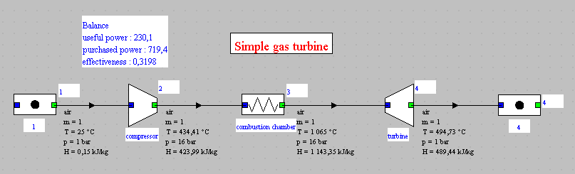
The gas turbine sucks air at 25 ° C and 1 bar, and compresses it to 16 bar in a 0.85 isentropic efficiency compressor.
The compressed air enters the combustion chamber burning natural gas, then the burnt gases are expanded in a turbine with a 0.85 isentropic efficiency.
The inlet temperature to the turbine is 1065 °C and combustion is assumed to be perfect.
Technological aspects
To achieve compression ratios r of 20 or 30, the compressor is multi-stage, sometimes with intermediate refrigeration intended to reduce the work consumed. The axial rotors consist of a stack of discs, either mounted on a central hub, or assembled in a drum around their periphery. The materials used range from aluminum or titanium alloys for the first stages to steel alloys and refractory alloys for the last stages, which can withstand temperatures reaching 500 °C.
The combustion chamber is normally constructed of a refractory alloy. Various types will be presented later.
In open cycle gas turbines, the main technological constraints lie in the first stages of the expansion turbine, which are subjected to the flow of exhaust gases at very high temperatures.
The most exposed parts are in particular the rotor blades, which are very difficult to cool and, moreover, particularly sensitive to abrasion. It is therefore important to use a very clean fuel (absence of particles and chemical components liable to form acids), and to limit the temperature according to the mechanical characteristics of the blades.
The materials used for the turbine blades are refractory alloys based on nickel or cobalt, and it is planned to use ceramics in the future.
Loading the model
The model is loaded by opening the diagram file and an appropriately configured project file.
Start by loading the model, then perform the other proposed activities.
Loading the model
Click on the following link: Open a file in Thermoptim
You can also:
- either open the "Project files/Example catalog" (CtrlE) and select model m3.3 in Chapter 3 model list.
- or directly open the diagram file (GT_light.dia) using the "File/Open" menu from the diagram editor menu, and the project file (GT_light.prj) using the "Project files/Load a project " menu from the simulator.
Discovery of Thermoptim
The diagram editor allows you to describe graphically and qualitatively the system studied. It includes a palette presenting the different representable components and a work panel where these components are placed and interconnected by vector links.
The simulator allows you to quantify and then calculate the model described in the diagram editor. It includes the lists of the different points, processes, nodes and exchangers of the model.
Display these two windows and study their content.
Refer for more explanations to the Thermoptim discovery exploration accessible from the menu at the top left of the browser screen.
Main components of the model
How many main components does the cycle use?
Mechanical energy
What component (s) put mechanical energy into play?
Energies put into play
Enter the values in the text fields below. Your answer is evaluated against the correct value, with an interval corresponding to a precision which depends on the question.
Remember that the energies or capacities received by a system are counted positively, and those it supplies to the outside are counted negatively. In Thermoptim screens, they are therefore positive or negative, depending on the case.
However, in these exercises, enter only the absolute values of the capacities involved (in kW)
Value of compression power?
Value of the power of the turbine?
Value of net mechanical power?
Value of the thermal power supplied to the machine?
Value of the efficiency?
Model settings
In this section, we will make the link between the model statement and the configuration of the main points and processes
Settings retained
The state of point 1 at the compressor inlet is known: temperature of 25 ° C and atmospheric pressure, assumed to be 1 bar to simplify things.
Open point 1 and examine its settings.
Its pressure is equal to 1 bar, and its temperature at 25 °C.
The air composition can be displayed by clicking on the button to the right of the substance name.
The compressor was set as follows: adiabatic, isentropic reference, isentropic efficiency equal to 0.85, and open system. Its compression ratio is calculated as the ratio of the pressure of the downstream point (2) to that of the upstream point (1). It is worth 16.
Open the "compressor" process, and examine its settings.
It connects point 1 and point 2, and its configuration is "adiabatic", "isentropic reference", with an isentropic efficiency equal to 0.85.
It is in point 2 that the pressure of 16 bar is defined.
Open point 2. Its setting is "unconstrained", which means that the pressure and its temperature are independent.
When the "compressor" process is calculated, the temperature of point 2 is determined.
If you change the pressure of point 2, for example by entering 20 bar, the new end of compression temperature is calculated. It differs from the previous one.
Combustion is not modeled as such in this simplified model. It is replaced by an "exchange" process which allows the temperature of the compressed air to be brought to 1065 °C. Its setting does not pose any particular problem.
Evolution (3–4) is an irreversible adiabatic expansion from 16 bar to 1 bar, with isentropic efficiency .
This evolution is modeled by the "turbine" process.
The upstream state of the fluid is that of point 3, the pressure and temperature of which are known.
For the downstream point, only the pressure is known.
Open the "turbine" process, and examine its setting.
It connects point 3 and point 4, and its setting is "adiabatic", "isentropic reference", with an isentropic efficiency equal to 0.85.
It is in point 4 that the outlet pressure of 1 bar is defined.
If you change the value of the isentropic efficiency, the new outlet temperature is calculated.
Cycle plot in the (h, ln (P)) chart
First step: loading the diagram of the air (h, ln (P)) chart
We will now study the cycle in the (h, ln (P)) chart, which allows you to read the enthalpies involved directly on the abscissa axis
Click this button
You can also open the diagram using the "Interactive Charts" line in the "Special" menu of the simulator screen, which opens an interface that links the simulator and the diagram. Double-click in the field at the top left of this interface to choose the type of diagram desired (here "Ideal gases").
Once the diagram is open, select "(h, p)" in the "Graph" menu, and click on the line "Load a base gas" in the Gas editor menu, and choose "air" from the protected compound gases.
If you do not have access to the (h, P) chart of the gas turbine, open the Help/Global settings menu in the Thermoptim simulator screen, check the "(h, P) chart for gas" option at the bottom on the left, then close the window by clicking on "OK".
Restart Thermoptim. The (h, P) charts should be displayable.
If the window is displayed correctly, but without showing the lines of iso-values in the chart, it is undoubtedly that the interval for displaying the values is not the right one, due to the previous settings.
It is possible to modify the calculation and display values by playing on the parameters in the chart menus:
- Open the Chart/X-axis menu line, then enter a minimum of -50 and a maximum of 1450 to define the values of the enthalpies to be displayed
- Open the Chart/Y-axis menu line, then enter a minimum of 1 and a maximum of 32 to define the values of the pressures to be displayed
- If the lines of iso-values are not the right ones, open the
menu line Chart/parameters, then enter the following values to
define the iso-values to be displayed:
- Temperatures between -50 °C and 1150 °C
- Pressures between 1 and 32 bar
Second step: loading a pre-recorded cycle corresponding to the loaded project, the layout of which has been previously refined in order to be more precise
Click this button
You can also open this cycle as follows: in the diagram window, choose "Load a cycle" from the Cycle menu, and select "GT_light_25Thin.txt" from the list of available cycles. Then click on the "Connected points" line in the Cycle menu.
Cycle analysis
Point 1 is close to the abscissa axis, at the intersection between the vertical isotherm T = 25 °C and the isobar P = 1 bar. The non-reversible adiabatic compression leads to point 2, on the isobar P = 16 bar.
The change in enthalpy between points 1 and 2 is proportional to the power consumed by the compressor.
The heating in the combustion chamber leads to point 3, at the intersection of the isobar P = 16 bar and the isotherm T = 1065 °C.
The change in enthalpy between points 2 and 3 is proportional to the power supplied to the combustion chamber.
Evolution (3–4) is a non-reversible adiabatic expansion from 16 bar to 1 bar. The change in enthalpy between points 3 and 4 is proportional to the power generated by the turbine.
Variation in performance when air temperature changes
The previous model assumed that the outside temperature was 25 °C.
We are now interested in the operation of the plant when the outside temperature is 35 °C.
Enter this value in point 1, then recalculate it.
Then recalculate several times in the simulator screen until the balance stabilizes.
Once the settings have been made, in order for the modifications to appear in the diagram editor, hide the values, then re-display them, by selecting the menu line "Special/Show values" twice, or by typing twice the F3 key.
Reduction in useful power
The increase in air temperature has the effect of reducing the useful power
For comparison, here are the performance values of the cycle with air temperature of 25 °C (first part of the exploration)
by what value does the useful power decrease?
by what value decreases the purchased power?
First law balance
what is the value of the compression power?
Power produced by the turbine
what is the value of the power produced by the turbine?
Efficiency value
what is the value of the efficiency?
Determination of isentropic efficiency when the state of the exit point is known
The initial model (T1 = 25 °C) assumed that the isentropic efficiency of the compressor was known.
We are now interested in the configuration of the model when we know not its value but that of the state of the exit point (425 °C, 16 bar).
Go back from the initial setting and enter these values in the screen of point 2, then recalculate it.
In the screen of the "compressor" process, select the option "Calculate the efficiency, the outlet point being known" at the bottom right, then recalculate the process.
What is the new value of the isentropic compression efficiency? (enter its value between 0 and 1)
It is thus possible to set compression or expansion knowing either its isentropic efficiency or the state of its outlet point.
Conclusion
This exploration allowed you to discover Thermoptim and to start using this software package to make settings for a simple model.
You can perform others to analyze the sensitivity of the model to various parameters, such as the isentropic efficiency of the turbine.
We recommend that you read the Thermoptim documentation, and in particular the first two volumes of its reference manual.
Other guided explorations will allow you to study variants of this cycle to improve performance.
Open the diagram editor and count the components of the model.
Please note: to answer this question, do not count the inputs and outputs of fluids among the components