Introduction

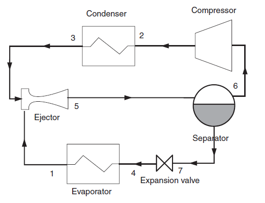
An ejector refrigeration cycle with compressor is as follows:

At the outlet of the condenser, the high pressure refrigerant in the liquid state is expanded as the driving fluid of the ejector and becomes two-phase, entraining and compressing the low pressure refrigerant leaving the evaporator.

The mixture leaving the ejector at intermediate pressure is then separated, the vapor phase being compressed at high pressure, and the liquid phase expanded without work and then directed to the evaporator

Reference cycle

The R134a reference cycle is the same as that used for the exploration on the total injection cycle: it operates between an evaporation pressure of 1 bar and a condenser pressure of 12 bar.

At the outlet of the evaporator, a flow rate $m=1g/s$ of fluid is entirely vaporized, with an overheating of 5 °C.

It is then compressed to 12 bar following an irreversible adiabatic compression. The actual compression is characterized by an isentropic efficiency, defined as the ratio of the work of the reversible compression to the real work. Its value is assumed to be 0.8.

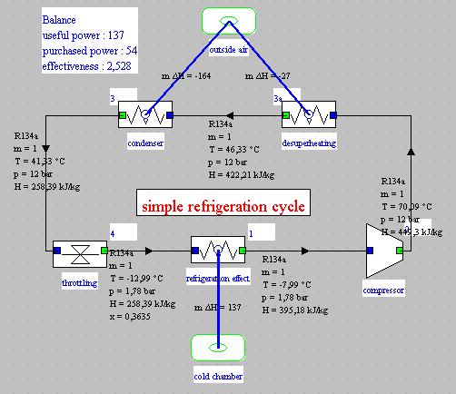
The cooling of the fluid in the condenser by exchange with the outside air involves two stages: desuperheating in the vapor zone followed by condensation, with sub-cooling of 10° C.

It is then expanded without work in a capillary, to the pressure of 1 bar.

The COP for such a cycle is worth 2.04.

Settings retained for the ejector cycle

The ejector refrigeration cycle operates between an evaporation pressure of 1 bar and a condenser pressure of 12 bar, the intermediate pressure being determined by the ejector.

At the outlet of the evaporator, the flow rate $m=1g/s$ de fluide est entièrement vaporisé, avec uof fluid is entirely vaporized, with a superheating of 5 °C.

The compressor is characterized by an isentropic efficiency assumed to be equal to 0.8.

The refrigerant is condensed without sub-cooling.

The only new setting is that of the ejector, which will be explained later.

The balance of the cycle shows a significant improvement in the COP which reaches the value of 2.36, or 18% better than that of the single-stage cycle. The cooling capacity is also increased, from 136 W to 203 W, due to the fact that the evaporator input quality is much lower.

Loading the model

Load the model

Click on the following link: Open a file in ThermoptimOpen a file in Thermoptim

Ejector settings

An ejector or injector receives as input two fluids normally gaseous but which may also be liquid or two-phase

• the high pressure fluid called primary or motive
• the low pressure fluid, called secondary fluid or aspirated

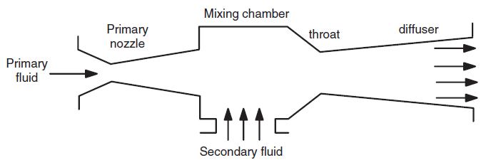
The primary fluid is accelerated in a converging-diverging nozzle, creating a pressure drop in the mixing chamber, which has the effect of drawing the secondary fluid. The two fluids are then mixed and a shock wave may take place in the throat. This results in an increase in pressure of the mixture and reduction of its velocity which becomes subsonic. The diffuser then converts the residual velocity in increased pressure.

The ejector thus achieves a compression of the secondary fluid at the expense of a decrease in enthalpy of the primary fluid.

The ejector model is implemented in an external class of Thermoptim. It is an external mixer.

Open the ejector screen, and calculate it.

It has four parameters:

• the factor $\mathrm{Pe}/\mathrm{Pb}$ of pressure drops at the entry of the secondary fluid into the ejector, which determines the minimum pressure in the ejector. It is worth 0.75 in our case.
• the friction factor to possibly take into account a pressure drop in the mixing zone. It is worth 1 here, which means that there is no pressure drop.
• 
  
• the isentropic efficiency of the two nozzles (working fluid and entrained fluid). It is worth 0.95 here.
• the isentropic efficiency of the outlet diffuser. It is worth 0.95 here.

These settings only play second order on the calculations, which mainly depend on the enthalpies of the two fluids.

The calculation results are displayed between the parameters input fields. The first line indicates:

• Pout, outlet pressure (bar)
• Temp, outlet temperature (°C)
• Pmi/Pd, ratio of the pressure of the working fluid to the outlet pressure
• Pd/Psi, ratio of the outlet pressure to the pressure of the entrained fluid
• quality, output quality
• DP, initial pressure drop of the entrained flow
• Pmix, mixing pressure (bar)

The second line provides the sections (in mm2) at the entrance to the mixing zone for the motor (Amb) and driven (Asb) fluids.

Cycle plot in the (h, ln (P)) chart

First step: loading the R134a (h, ln (P)) chart

Click this button

Second step: loading a pre-recorded cycle corresponding to the loaded project

Click this button

The cycle appears in blue. A distinction is made between the two LP and HP circuits.

Simple cycle overlay

Click this button

What is particularly remarkable is the very strong increase in the useful effect, due to the fall in the quality at the inlet of the evaporator.

Application exercise

Study of the influence of subcooling

In this model, no sub-cooling was taken into account at the condenser outlet.

Conclusion

This exploration allowed you to study a model of an ejector refrigeration installation.

Note that one of the practical problems encountered when using an ejector in a cycle is that its performance depends very much on its operating conditions: the compression ratio obtained is obviously a function of the drive ratio, but a variation of the latter induces a modification of the optimal geometry of the ejector, which it is obviously impossible to achieve.

IIt follows that an ejector does not adapt well enough to operation outside the design conditions.