Introduction
The objective of this exploration is to guide you in your first steps of using Thermoptim, by making you discover the main screens and functionalities associated with a simple refrigeration installation model.
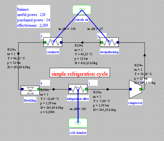
You will discover the layout of the screens of the points and the processes, the way in which they can be reparametered and calculated, the concepts of useful and paying energies making it possible to draw up the global energy balances and to determine the Coefficient of Performance COP.
You will visualize the cycles in the thermodynamic diagram (h, ln (P)) and you will carry out studies of sensitivity of the cycle to the outside temperature and the high pressure. You will analyze the interest of sub-cooling.
In a vapor compression refrigeration installation, one seeks to maintain a cold enclosure at a temperature below ambient.
The principle consists in evaporating a refrigerant at low pressure (and therefore low temperature), in an exchanger in contact with the cold enclosure.
For this, the evaporation temperature of the refrigerant must be lower than that of the cold enclosure. The fluid is then compressed to a pressure such that its condensation temperature is higher than room temperature.
It is then possible to cool the fluid by heat exchange with the ambient air, until it becomes liquid. The liquid is then expanded by isenthalpic lamination to low pressure, and directed into the evaporator. The cycle is thus closed.
Setting retained
The compression refrigeration cycle of R134a operates between an evaporation pressure of 1.78 bar and a condenser pressure of 12 bar.
At the outlet of the evaporator, a flow rate of fluid is entirely vaporized, with an superheating of 5 °C.
It is then compressed to 12 bar following an irreversible adiabatic compression. The actual compression is characterized by an isentropic efficiency, defined as the ratio of the work of the reversible compression to the real work. Its value is assumed to be 0.75
The cooling of the fluid in the condenser by exchange with the outside air involves two stages: desuperheating in the vapor zone followed by condensation.
It is then expanded without work in a capillary, up to the pressure of 1.78 bar.
Model loading
The model is loaded by opening the diagram file and an appropriately configured project file.
Start by loading the model, then complete the three proposed activities.
Model loading
Click on the following link: Open a file in Thermoptim
You can also:
- either open the "Project files/Example catalog" (CtrlE) and select model m3.4 in Chapter 3 model list.
- or directly open the diagram file (refrig_light.dia) using the "File/Open" menu in the diagram editor, and the project file (refrig_light.prj) using the "Project file/Load" menu project in the simulator window.
Discovery of Thermoptim
The diagram editor allows you to describe graphically and qualitatively the system studied. It includes a palette presenting the different representable components and a work panel where these components are placed and interconnected by vector links.
The simulator allows you to quantify and then calculate the model described in the diagram editor. It includes the lists of the different points, processes, nodes and exchangers of the model.
Display these two windows and study their content.
Refer for more explanations to the Thermoptim discovery exploration accessible from the menu at the top left of the browser screen.
Main components of the model
How many main components does the cycle use?
Mechanical energy
What component (s) involve mechanical energy?
Energies put into play
Enter the values in the text fields below. Your answer is evaluated against the correct value, with an interval corresponding to a precision which depends on the question.
Remember that the energies or capacities received by a system are counted positively, and those it supplies to the outside are counted negatively. In Thermoptim screens, they are therefore positive or negative, depending on the case.
However, in these exercises, enter only the absolute values of the capacities involved (in W)
Value of the cooling capacity?
Value of compression power?
Settings retained
In this section, we will make the link between the model statement and the configuration of the main points and processes
At point 1 at the evaporator outlet, the refrigerant is in the vapor state superheated by 5 °C, at a temperature of about -8 °C. The pressure of R134a is 1.78 bar.
Open point 1 and examine its setting.
Its pressure is equal to 1.78 bar, and the option "set the saturation temperature" was chosen, with a Tsat approach of 5 °C.
The point being in the state of vapor, its quality is equal to 1.
Recall that, for a pure substance with liquid-vapor equilibrium, the quality is defined as the mass of vapor divided by the total mass of liquid and vapor.
If you change the pressure value, and you recalculate the point, its temperature is automatically modified.
The compressor compresses the refrigerant to 12 bar.
Open the "compressor" process, and examine its setting.
It connects point 1 and point 2, and is set as "adiabatic", "isentropic reference", with an isentropic efficiency equal to 0.75.
It is in point 2 that the pressure of 12 bar is defined.
Open point 2. Its setting is "unconstrained", which means that the pressure and its temperature are independent.
When the "compressor" process is calculated, the temperature of point 2 is determined.
If you change the pressure of point 2, for example by entering 10 bar, the new compressor outlet temperature is calculated. It differs from the previous one.
The cooling of the fluid in the condenser by exchange with the outside air has two stages:
- desuperheating (2–3a) in the vapor zone
- followed by condensation (3a–3).
Points 3a et 3 are located at the intersection of the saturation curve and the isobar P = 12 bar, or, which comes to the same thing, the isotherm T = 47 ° C. Point 3a is located on the right, at the limit of the vapor zone, and point 3 on the left, at the limit of the liquid zone.
Point 3a is set up in a completely analogous way to point 1, the option "set the saturation temperature" being chosen, and the quality being equal to 1, to indicate the state of vapor.
Point 3 is set analogously, with the proviso that the quality is 0, to indicate the liquid state.
The process (3–4) is an expantion without work, and therefore isenthalpic, from 12 bar to 1.78 bar.
This evolution is modeled by the "throttling" process.
The upstream state of the fluid is that of point 3, the pressure and temperature of which are known.
For the downstream point, the pressure and the enthalpy are known, so that Thermoptim can calculate its state.
It is in point 4 that the outlet pressure of 1.78 bar is defined.
The outlet state is two-phase, which means that the temperature is equal to that of saturation at this pressure. The quality, equal to 0.4, is determined when calculating the process.
The useful capacity is the heat extracted at the evaporator (129 W), and the purchased power the work provided to the compressor (54 W). The ratio of the two being greater than 1, the term of efficiency is no longer suitable.
This is why we speak of the cycle coefficient of performance (COP).
What is the COP value of this cycle
Cycle plot in the (h, ln (P)) chart
First step: loading the R134a (h, ln (P)) chart
Click this button
You can also open the diagram using the "Interactive Diagrams" line in the "Special" menu of the simulator screen, which opens an interface that links the simulator and the diagram. Double-click in the field at the top left of this interface to choose the type of diagram desired (here "Vapors")..
Once the diagram is open, choose "R134a" from the substance menu, and select "(h, p)" from the "Chart" menu.
Second step: loading a pre-recorded cycle corresponding to the loaded project, the layout of which has been previously refined in order to be more precise
Click this button
You can also open this cycle as follows:
- in the diagram window, choose "Load a cycle" from the Cycle menu
- and select "refrig_lightEnThin.txt" from the list of available cycles.
- Then click on the "Connected points" line in the Cycle menu.
Identification of some characteristic points in the diagram
What is the point in the liquid zone?
What is the point in two-phase zone?
What is the point with the highest temperature?
Modifications of the cycle taking into account a sub-cooling of 10 ° C
Loading the model
Click on the following link: Open a file in Thermoptim
You can also:
- either open the "Project files/Example catalog" (CtrlE) and select model m3.5 in Chapter 3 model list.
- or directly open the diagram file (refrig_light_SC10.dia) using the "File/Open" menu in the diagram editor, and the project file (refrig_light_SC10.prj) using the "Project file/Load" menu project in the simulator window.
Cycle display with subcooling
The loading of the cycle with sub-cooling drawn in blue makes it possible to superimpose it on the initial cycle. In the (h, ln (P)) chart, the increase in the cooling effect is clearly visible.
Click this button
You can also open this cycle as follows: in the diagram window, choose "Load a cycle" from the Cycle menu, and select "refrig_lightEnSC10Thin.txt" from the list of available cycles. Then click on the "Connected points" line in the Cycle menu.
Increase in useful effect
Subcooling increases the useful effect.
For comparison, here are the performance values of the machine cycle without subcooling (first part of the exploration).
How much does the cooling effect increase?
How much does the compression power increase?
First law balance
What is the value of the cooling capacity?
Compression power value
What is the value of the compression power?
COP value
What is the value of the COP?
Subcooling limit
A cold source is needed to cool the refrigerant.
In this example, we will assume that the exchange takes place with the outside air at 32 ° C.
What is the limit of the subcooling value?
Elimination of the sub-cooling cycle
For the rest of the scenario, we erase the sub-cooling cycle
Click this button
You can also delete the unnecessary cycle by following these steps: Display the Cycle manager from the Cycle menu. Click on the "Update cycle table" button, and deselect the row that you do not want to appear on the chart.
Variation in performance when the external temperature varies
The initial model assumed that the refrigerator was placed in a room at 32 ° C, which corresponds to a summer situation.
We are now interested in its use in winter in a kitchen whose temperature is 18 ° C.
The new corresponding project is loaded, without sub-cooling.
Loading the model
Click on the following link: Open a file in Thermoptim
You can also:
- either open the "Project files/Example catalog" (CtrlE) and select model m3.6 in Chapter 3 model list.
- or directly open the diagram file (refrig_light18.dia) using the "File/Open" menu in the diagram editor, and the project file (refrig_light18.prj) using the "Project file/Load" menu project in the simulator window.
energies put into play
For comparison, here are the performance values of the machine cycle without subcooling (first part of the exploration).
As you can see, the temperature change has a strong influence on the performance of the machine, and especially on the compression power.
What is the value of the cooling capacity?
What is the value of the compression power?
What is the COP value?
Plot of the two cycles in the (h, ln (P)) chart
Overlay of the two cycles in the diagram, the new cycle being drawn in red.
Click this button
You can also open this cycle as follows:
- in the diagram window, choose "Load a cycle" from the Cycle menu
- select "refrig_light18Thin.txt" from the list of available cycles
- Then click on the "Connected points" line in the Cycle menu.
The reduction in compression work and the increase in useful effect are clearly visible.
Application exercises
Now that you have finished this exploration, you can start from the loaded example, corresponding to the outside temperature of 18 ° C, and reset it to find for yourself the results that were obtained previously by loading the examples of directed exploration.
Once the settings have been made, in order for the modifications to appear in the diagram editor, hide the values, then re-display them, by selecting the menu line "Special/Show values" twice, or by typing twice the F3 key.
Sub-cooling
study of sub-cooling for Tex = 18 °C
Determine by yourself the maximum subcooling that can be obtained for this outside temperature, and deduce from this the performance of the cycle
Setting for Text = 25 °C
Set the cycle with a condensing pressure equal to 9.1 bar, which corresponds to Text = 25 ° C, and calculate the enthalpy balance.
Determination of isentropic efficiency when the state of the exit point is known
The previous model assumed that the isentropic efficiency of the compressor was known.
We are now interested in the configuration of the model when we know not its value but that of the state of the exit point (67 ° C, 12 bar).
Enter these values in the screen for point 2, then recalculate it.
In the screen of the "compressor" process, select the option "Calculate the efficiency, the outlet point being known" at the bottom right, then recalculate the process.
what is the new value of the isentropic compression efficiency? (enter its value between 0 and 1)
It is thus possible to set a compression knowing either its isentropic efficiency, or the state of its outlet point.
Conclusion
This exploration allowed you to discover Thermoptim and to start using this software package to make settings for a simple model.
You can perform others to analyze the sensitivity of the model to various parameters, such as the isentropic efficiency of the compressor.
We recommend that you read the Thermoptim documentation, and in particular the first two volumes of its reference manual.
Other guided explorations will allow you to study variants of this cycle to improve performance, especially two-stage cycles.
Finally, you can model a heat pump, which uses a cycle similar to the one you have just studied, the useful effect of which is no longer the cooling in the evaporator but the heat rejected in the condenser.
Open the diagram editor and count the components of the model, excluding external sources.
This question has several answers, depending on whether we consider multizone exchangers as composed of one or more components