Presentation of the exercise

This exercise is primarily intended to illustrate how to calculate adiabatic compressions and expansions. It is centered around the study of a small capacity gas turbine, called micro-turbine. This micro-turbine is an existing machine, used for several applications, including cogeneration.

In session S46En we will give a cogeneration facility example based on this machine.

This exercise is divided into three parts:

• in this part (session S21En) we assume that the machine is traversed by a single gas, air, initially modeled as a perfect gas, and in a second time as an ideal gas. The resulting model is obviously simplistic, but it is interesting for beginners, because it allows them to make the connection between analytical theoretical calculations and resolution in Thermoptim.
• in the second part (session S22En), we consider the combustion reaction that takes place in industrial machines. The model is much more realistic. The comparison with the analytical model allows us to analyze its limits
• in the third part(session S23En), we analyze quantitatively the irreversibilities of the cycle by setting up its exergy balance, and deduce ways of improving the machine cycle (regeneration).

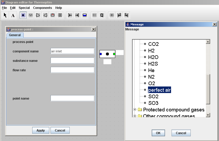
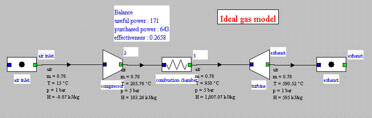
Before starting working with Thermoptim, we strongly recommend that you study session S07En_init, which introduces all the concepts which you will be using.

GT exercise

• gas turbine
• inlet conditions: 15 °C, 1 bar
• Intake air flow: 0.78 kg/s
• compression ratio: 5
• compression isentropic efficiency: 0.875
• turbine inlet temperature: 950 °C
• expansion isentropic efficiency: 0.885
• perfect air

Opening of Thermoptim

• two screens at opening
• diagram editor
• simulator

Thermoptim

Thermoptim

Thermoptim

Thermoptim

• gas turbine diagram
• air inlet
• compressor
• combustion chamber
• turbine
• fluid exhaust

Thermoptim

• diagram simulator interface

Thermoptim

Setting the model

When the simulator elements are created, Thermoptim initializes all the points with a pressure of 1 bar and a temperature of 300 K, which must then be modified according to the data of the problem you are studying.

The two steps that follow will show you how to set points and processes, then the next will remind you of the values that you should enter in Thermoptim.

Point settings

• double-click on a link (arrow) on a line of the point table
• thermodynamic state of a small volume of matter

Process settings

• double-click on a component
• change of fluid state, for a given flow-rate

Setting the parameters of points and processes

Set now the parameters of the various points one by one, checking that you enter the values of the temperatures known (T1, T3), as well as those of the pressures, as Thermoptim does not set them automatically. In order to do that, follow these steps:

• open point air inlet, enter a temperature of 15 °C and a pressure 1bar, then click on “Calculate”
• then open point 2, enter a pressure of 5 bar, and click on “Calculate”
• open point 3 and enter a temperature of 950 ° C and a pressure of 5 bar, and calculate it

It is not necessary to reset the point 4, since its pressure is 1 bar default and that its temperature will be recalculated later.

Set then the process’s parameters, for which default options are valid : the compression and the expansion are adiabatic, calculated with the isentropic reference, and their isentropic efficiencies are known. In order to do that, follow these steps:

• open process “compressor”, and enter an isentropic efficiency of 0.875, then click on “Calculate”, which sets the temperature of point 2 (207.14 °C).
• open process “combustion chamber”, and click on “Calculate”. The temperatures of its inlet and outlet points being known, the heat involved is calculated.
• open process “turbine”, and enter an isentropic efficiency of 0.885, then click on “Calculate”, which determines the temperature of point 4 (551.14 °C).

The calculation of the overall balance requires to understand the notion of energy type, explained in the next step.

Choice of the energy type

• double-click on the energy type field

Balance and synoptic view

Cycle on (T,s) chart

• chart-simulator interface

Cycle on (T,s) chart

Cycle on (T,s) chart

Chart-simulator interface

Cycle on (T,s) chart

Cycle on (T,s) chart

Cycle on (T,s) chart

Comparison with Carnot cycle

Comparison with an analytical perfect gas model

This session enabled you to build a simplified model of gas turbine, where the machine is traversed by air assumed to be perfect, and plot the cycle in the entropy chart.

A qualitative comparison with the Carnot cycle has allowed us to understand why the cycle efficiency is low. A further quantitative analysis will be made ​​in a later lesson (session S23En).

On this occasion, you could start learning to use Thermoptim. To master this tool, we recommend you browse its various reference manuals, available in the software documentation.

You can now compare the results obtained with an analytical solution which is possible given the assumptions made​​. The analytical solution and Thermoptim project and diagram files are provided in the attached archive.

As you can see, the model built in Thermoptim leads to exactly the same results as the analytical approach.

In the remainder of this session, you refine the model by replacing perfect air by ideal gas, so you can see the influence of the hypothesis on the fluid.

In another session (S22En), you will introduce a real combustion chamber, leading to a much more realistic model.

• Perfect gas model solution (zip, 71 Kb)

Modification of the perfect gas model

To replace the perfect air by air modeled as an ideal gas, we will use a feature that allows Thermoptim to simultaneously replace a substance in the set of points to which it is connected, and to update the simulator as well as the diagram editor.

Thermoptim

Balance and synoptic view

Comparison with the perfect gas model

You can now compare the results with those of the previous model (perfect gas).

The following table summarizes the results:

• in terms of net mechanical power, the error of the perfect gas model (PG) is 5% from the ideal gas model (IG)
• in terms of thermal power provided to the cycle it is 9.3%
• the error on efficiency is 4.7%
• the error on the temperature difference in the compressor is much lower than in the turbine, where it reaches 11%

• Ideal gas model solution (zip, 2 Kb)
• Model construction and verification methodology (pdf, 96 Kb)