Presentation
This session is the second part of an introductory course on heat integration or pinch method.
It presents in details a practical example of this method, with the heat exchanger network determination.
If you are not yet familiar with the basic concepts of heat integration (pinch, composites, algorithm for minimizing the pinch), we suggest you should first study session IT1En.
(Session realized on 01/09/11 by Renaud Gicquel)Gourlia case study
- Build the composite curves by hand
- Build the heat exchanger network by hand
- Solve the problem with Thermoptim
Problem data
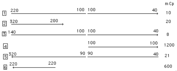
- Heat availability
| Stream 1 | 220 – 40 °C | 1,800 kW |
|---|---|---|
| Stream 2 | 320 – 200 °C | 2,400 kW |
| Stream 3 | 140 – 40 °C | 800 kW |
| Stream 4 | 100 °C | 1,200 kW |
| Boiler | 600 °C | 1,900 kW |
Problem data
- Needs
| Stream 5 | 40 – 320 °C | 6,000 kW |
|---|---|---|
| Stream 6 | 220 °C | 600 kW |
Problem Table Algorithm PTA
-
1) shift minimal and maximal temperatures by ΔTmin/2
- decrease for hot streams
- increase for cold streams
- 2) determine the temperature intervals of the problem by sorting the bounds of the upper and lower temperatures of each stream and build the enthalpy balances of each temperature interval which determines the hot and cold composites
- 3) sum up the enthalpy deficits
- 4) bring as hot utility the equivalent value of the maximum enthalpy deficit
PTA: 1) temperature shift
- before
stream m Cp Ts Tt H (kW/K) (°C) (°C) (kW) 1 10 40 220 1,800 2 20 200 320 2,400 3 8 40 140 800 4 1200 100 101 1,200 5 21 40 320 6,000 6 600 220 221 600 - after
stream m Cp type Tinf Tsup Δh (kW/K) (°C) (°C) (kW) 1 10 chaud 35 215 1,800 2 20 chaud 195 315 2,400 3 8 chaud 35 135 800 4 1200 chaud 95 96 1,200 5 21 froid 45 325 6,000 6 600 froid 225 226 600
PTA: 2) temperature intervals
-
1) shift minimal and maximal temperatures by ΔTmin/2
- decrease for hot streams
- increase for cold streams
- 2) determine the temperature intervals of the problem by sorting the bounds of the upper and lower temperatures of each stream and build the enthalpy balances of each temperature interval which determines the hot and cold composites
- 3) sum up the enthalpy deficits
- 4) bring as hot utility the equivalent value of the maximum enthalpy deficit
PTA: 2) temperature intervals
- Δhbd = (Ti - Ti+1) (ΣmCpb - ΣmCpd) = Δhb - Δhd
| interval | Ti | Ti + 1 | streams | Ti - Ti + 1 | Σ(m Cp) | ΔHbd |
|---|---|---|---|---|---|---|
| (°C) | (°C) | (K) | (kW) | (kW) | ||
| 1 | 325 | 315 | *5* | 10 | 21,43 | 214 |
| 2 | 315 | 226 | *5,2* | 89 | 1,43 | 127 |
| 3 | 226 | 225 | *5,2,6* | 1 | 601,43 | 601 |
| 4 | 225 | 21 | *5,2* | 10 | 1,43 | 14 |
| 5 | 215 | 195 | *5,2,1* | 20 | -8,57 | -171 |
| 6 | 195 | 135 | *5,1* | 60 | 11,43 | 686 |
| 7 | 135 | 96 | *5,1,3* | 39 | 3,43 | 134 |
| 8 | 96 | 95 | *5,1,3,4* | 1 | -1196,6 | -1197 |
| 9 | 95 | 45 | *5,1,3* | 50 | 3,43 | 171 |
| 10 | 45 | 35 | *1,3* | 10 | -18,0 | -180 |
PTA: 3) cumulative net enthalpy balances
-
1) shift minimal and maximal temperatures by ΔTmin/2
- decrease for hot streams
- increase for cold streams
- 2) determine the temperature intervals of the problem by sorting the bounds of the upper and lower temperatures of each stream and build the enthalpy balances of each temperature interval which determines the hot and cold composites
- 3) sum up the enthalpy deficits
- 4) bring as hot utility the equivalent value of the maximum enthalpy deficit
PTA: 3) cumulative net enthalpy balances
| interval | Ti | Ti + 1 | ΔHbd | sum |
|---|---|---|---|---|
| (°C) | (°C) | (kW) | (kW) | |
| 1 | 325 | 315 | 214 | -214 |
| 2 | 315 | 226 | 127 | -341 |
| 3 | 226 | 225 | 601 | -943 |
| 4 | 225 | 21 | 14 | -957 |
| 5 | 215 | 195 | -171 | -786 |
| 6 | 195 | 135 | 686 | -1471 |
| 7 | 135 | 96 | 134 | -1,605pinch |
| 8 | 96 | 95 | -1,197 | -409 |
| 9 | 95 | 45 | 171 | -580 |
| 10 | 45 | 35 | -180 | -400 |
PTA: 4) enthalpy balances with input
-
1) shift minimal and maximal temperatures by ΔTmin/2
- decrease for hot streams
- increase for cold streams
- 2) determine the temperature intervals of the problem by sorting the bounds of the upper and lower temperatures of each stream and build the enthalpy balances of each temperature interval which determines the hot and cold composites
- 3) sum up the enthalpy deficits
- 4) bring as hot utility the equivalent value of the maximum enthalpy deficit
PTA: 4) enthalpy balances with input
| interval | Ti | Ti + 1 | Δh net | 1605 |
|---|---|---|---|---|
| (°C) | (°C) | (kW) | ||
| 1 | 325 | 315 | 214 | 1391 |
| 2 | 315 | 226 | 127 | 1264 |
| 3 | 226 | 225 | 601 | 662 |
| 4 | 225 | 21 | 14 | 648 |
| 5 | 215 | 195 | -171 | 819 |
| 6 | 195 | 135 | 686 | 134 |
| 7 | 135 | 96 | 134 | 0 |
| 8 | 96 | 95 | -1197 | 1196 |
| 9 | 95 | 45 | 171 | 1025 |
| 10 | 45 | 35 | -180 | 1205 |
Stream pairing
- Notations
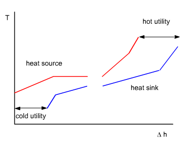
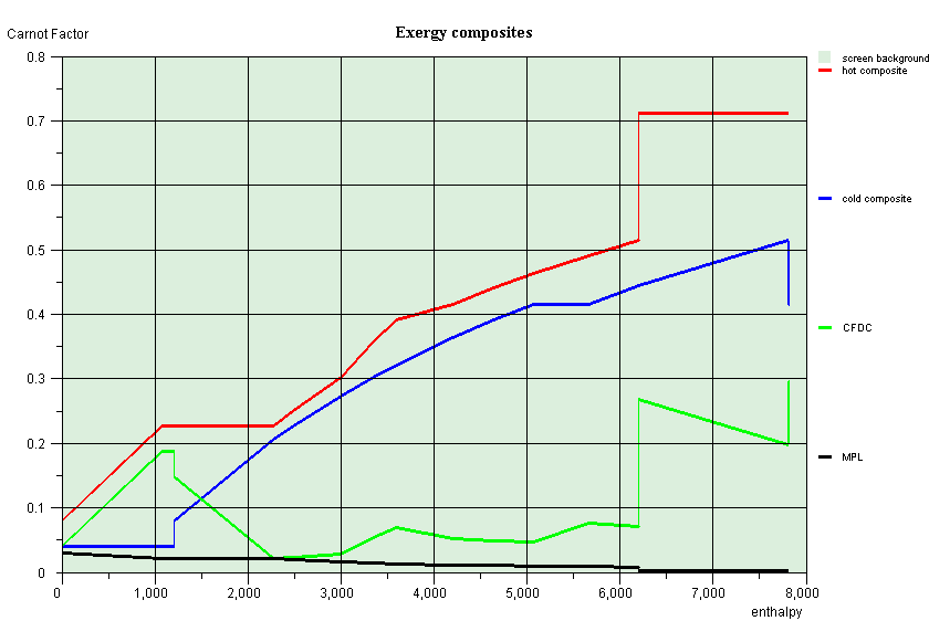
Composite curves
- The pinch separates the problem in two parts
- Each zone is thermally independant
- Heat exchanger networks can be built separately
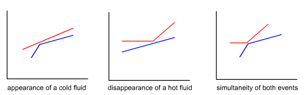
Conditions for a pinch to appear
- Pinch:
- either appearance of a new cold stream (need)
- or disappearance of a hot stream (availability)
- or simultaneity of both events: onset of a cold stream and disappearance of a hot stream
Rules
- separately endo- and exothermic zones study
- begin the design at the pinch and depart gradually from it, to deal first with the most constrained problem
- maximize the load of heat exchangers (to minimize their number)
- above the pinchmCph ≤ mCpc
- below the pinch mCph ≥ mCpc
Stream pairing
- Reminder of data
Above the pinch
- the first interval of the endothermic zone: hot stream 4 disappearance
- 1 cold stream (5), and 2 hot streams (1 and 3)
- mCp constraints are met
- we must then split (5) in two
Above the pinch
- interval above:
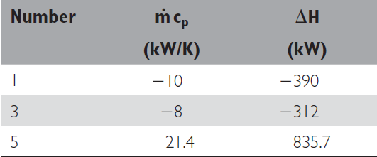
number mCp ΔH (kW/K) (kW) 1-10 600 5 21.4 1,285.7 - disappearance of stream 3
- the corresponding load (320 kW) must be supplied to stream 5: mCp52 = mCp3 = 8
Above the pinch
- we deduce mCp51 = 13.4
- to exhaust stream 1 (1,200 kW), the exit temperature of heat exchanger 1 is equal to 179°C
Above the pinch
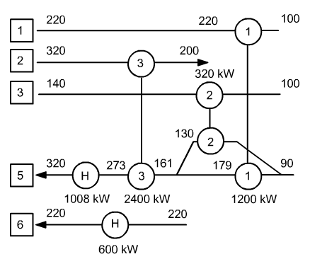
- streams 1 and 3 being exhausted, only 2 still contains availability (2,400 kW), which must be shared between the divided stream 5 and stream 6
- we can transfer the entire load in 6 (600 kW), and part of the residual load on the first branch of 5 (1,800 kW of the 1,888 required). However, this scenario leads to a failure in terms of T
- better to remix both stream 5 branches at the outlet of heat exchangers 1 and 2, and to have a hot utility (1,608 kW)
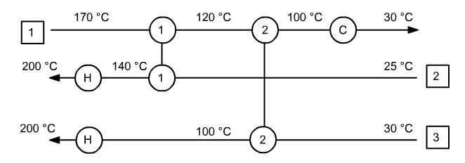
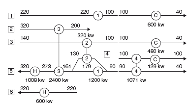
Heat exchanger network
- Hot end
Below the pinch
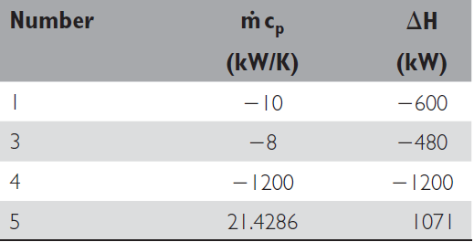
- only one cold stream: 5
- constraint mCph ≥ mCpc met if and only if paired to 4
- by maximizing the load of this exchanger (5), and knowing that the inlet T of 5 is 40 °C:
- Δh5 = mCp5 (90 - 40) = 1,071 kW
Below the pinch
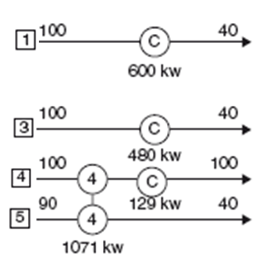
- 5 totally heated
- cannot cool 1, 3, and4
- to be done by cold utilities (1,209 kW)
Final heat exchanger network
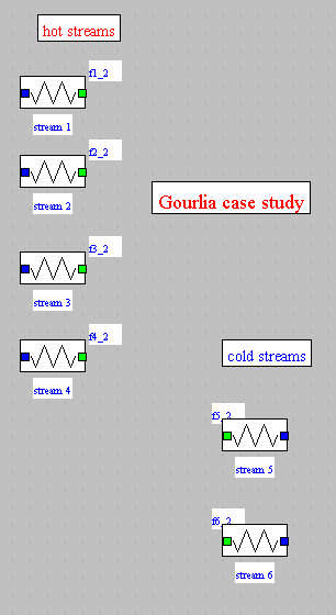
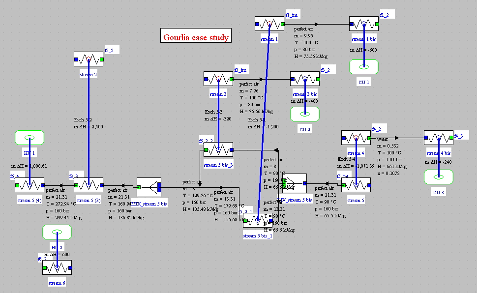
Modeling with Thermoptim
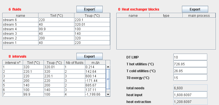
- Assumptions
- fluids : perfect air and steam
-
estimated flow rates :
m ΔH (kg/s) (kW) stream 1 9.946 -1,800 stream 2 19.892 -2,400 stream 3 7.9568 -800 stream 4 0.5317 -1,200 stream 5 21.312 6,000 stream 6 0.3232 600
Modeling tips
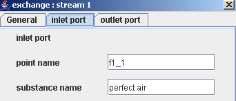
- enter data in both the inlet and outlet tabs
- pinch method fluid
- ΔTpinc = 10 K

Optimization screen
Composites
Heat exchanger network
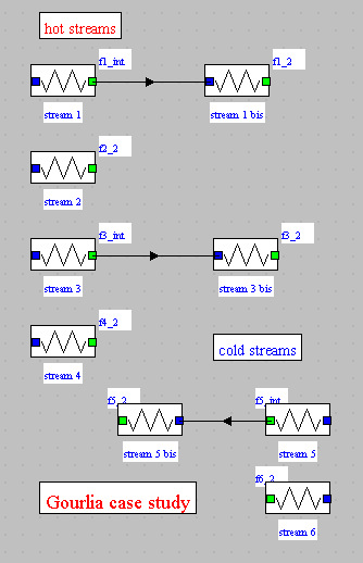
- 1) divide all streams that cross the pinch, in order to separate both sub-networks
Heat exchanger network
- 2) analyze the heat capacity rates mCp of the streams

Heat exchanger network
- 3) build exchange blocks to test possible matches:
- parallelization of 5 above the pinch
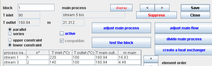
Heat exchanger network
- 4) build the exchangers :
- beware of streams duplicated
- exchangers are not automatically built in the diagram editor
Small practical difficulties
- 1) model modification:
- division of streams across the pinch
- exchangers not built in the diagram editor
- 2) default parallelizations may not be satisfactory
- 3) in exchangers, the quality of recalculated outlet points should not be between 0 and 1 (evaporation and condensation)
- Therefore: operate step by step creating backup project and diagram files
Full heat exchanger network
Practical use of the pinch method
In this session, we have illustrated the heat integration method by treating an example proposed in 1989 by Gourlia in the Revue Générale de Thermique.
Thermoptim files of the example can be downloaded from the link below.
We now suggest that you refer to the specialized temperature, and in particular to publications of Prof. B. Linnhoff.
We recommend that you read the following synthesis:
Introduction to Pinch Technology, Copyright 1998 Linnhoff March.